R6 class ModelCompareUnivariate

R6 class ModelCompareUnivariate

R6 class ModelCompareUnivariate

Super class

tswgewrapped::ModelCompareBase -> ModelCompareUnivariate

Methods

Public methods

• ModelCompareUnivariate$new()

• ModelCompareUnivariate$get_data_var_interest()

• ModelCompareUnivariate$plot_multiple_realizations()

• ModelCompareUnivariate$evaluate_residuals()

• ModelCompareUnivariate$summarize_build()

• ModelCompareUnivariate$clone()

Inherited methods

• tswgewrapped::ModelCompareBase$add_models()

• tswgewrapped::ModelCompareBase$compute_metrics()

• tswgewrapped::ModelCompareBase$get_batch_size()

• tswgewrapped::ModelCompareBase$get_data()

• tswgewrapped::ModelCompareBase$get_model_names()

• tswgewrapped::ModelCompareBase$get_n.ahead()

• tswgewrapped::ModelCompareBase$get_tabular_metrics()

• tswgewrapped::ModelCompareBase$keep_models()

• tswgewrapped::ModelCompareBase$plot_batch_ases()

• tswgewrapped::ModelCompareBase$plot_batch_forecasts()

• tswgewrapped::ModelCompareBase$plot_boxplot_ases()

• tswgewrapped::ModelCompareBase$plot_simple_forecasts()

• tswgewrapped::ModelCompareBase$remove_models()

• tswgewrapped::ModelCompareBase$set_batch_size()

• tswgewrapped::ModelCompareBase$set_verbose()

• tswgewrapped::ModelCompareBase$statistical_compare()

---

Method new()

Initialize an object to compare several Univatiate Time Series Models

Usage

ModelCompareUnivariate$new(
  data = NA,
  var_interest = NA,
  mdl_list,
  n.ahead = NA,
  batch_size = NA,
  step_n.ahead = TRUE,
  verbose = 0
)

Arguments

data

A Univariate Time Series Realization

var_interest

If data is a dataframe with multiple columns, then what is the output variable of interest

mdl_list

A named list of all models (see format below)

n.ahead

The number of observations used to calculate ASE or forecast ahead

batch_size

If any of the models used sliding ase method, then this number indicates the batch size to use

step_n.ahead

If using sliding window, should batches be incremented by n.ahead (Default = TRUE)

verbose

How much to print during the model building and other processes (Default = 0)

Returns

A new `ModelCompareUnivariate` object.

---

Method get_data_var_interest()

Returns the dependent variable data only

Usage

ModelCompareUnivariate$get_data_var_interest()

Returns

The dependent variable data only

---

Method plot_multiple_realizations()

Creates multiple realization of each model. Useful to check model appropriateness.

Usage

ModelCompareUnivariate$plot_multiple_realizations(
  n.realizations = 4,
  lag.max = 25,
  seed = NA,
  plot = c("all"),
  scales = "free_y"
)

Arguments

n.realizations

Number of realization to create (Default: 4)

lag.max

lag.max to plot for ACF (Default: 25)

seed

The seed to use for generating realizations

plot

A vector of options to plot (Default = c("all")) Other options: 'realization', 'acf', 'spectrum'

scales

The scales argument to be passed to ggplot facet_wrap layer (Default = 'free_y') Other appropriate options: 'fixed'

---

Method evaluate_residuals()

For the models for which the residuals have been provided, this method will check whetehr the residuals are white noise or not. (1) Plots the residuals and the ACF values (2) Performs the Ljung-Box test for K = 24 and K = 48

Usage

ModelCompareUnivariate$evaluate_residuals(lag.max = 50)

Arguments

lag.max

The maximum lag to plot for the ACF

Returns

A dataframe containing the results of the 2 Ljung-Box tests

---

Method summarize_build()

Not applicable for the Univariate Compare, since we are passing already build models

Usage

ModelCompareUnivariate$summarize_build()

---

Method clone()

The objects of this class are cloneable with this method.

Usage

ModelCompareUnivariate$clone(deep = FALSE)

Arguments

deep

Whether to make a deep clone.

Examples

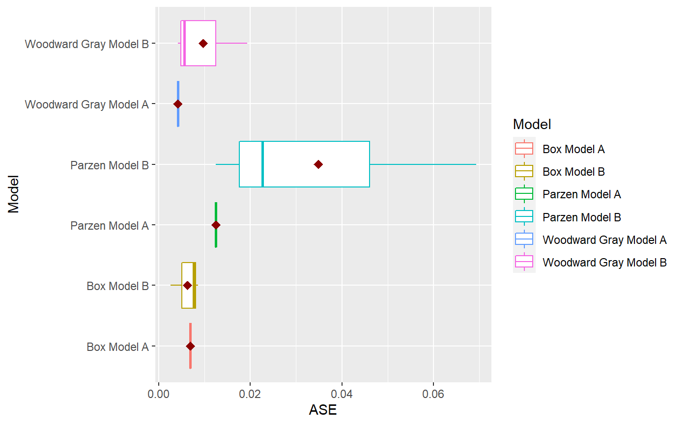
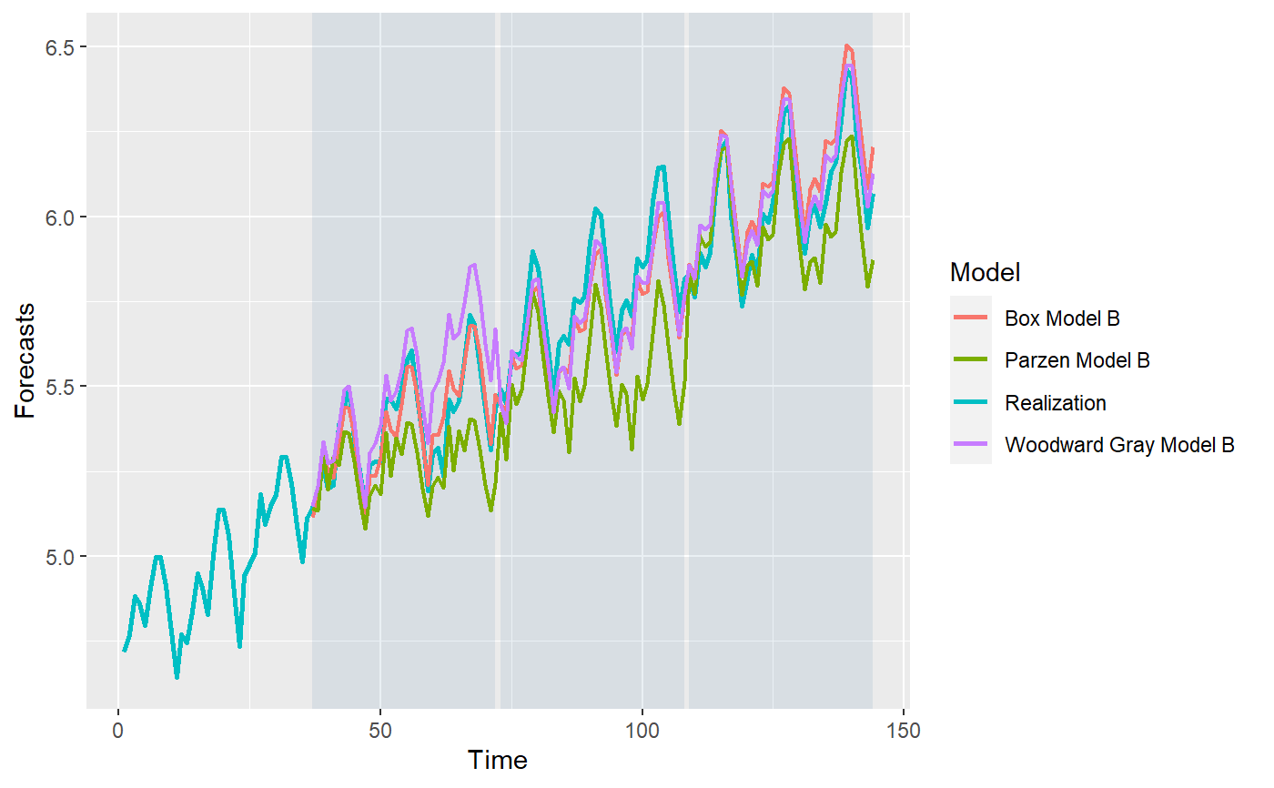
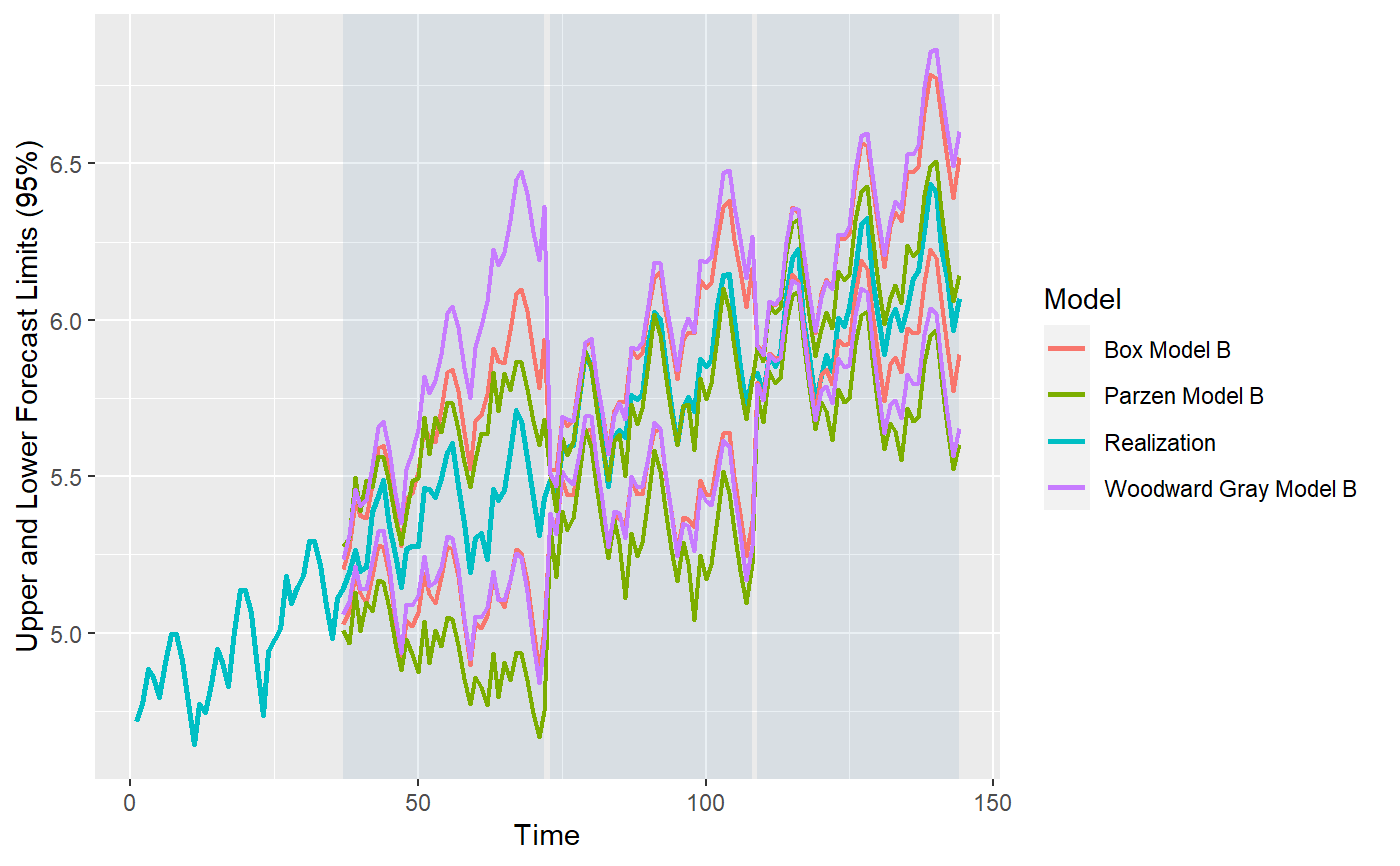
library(tswge)
data("airlog")

# Woodward Gray Airline Model
phi_wg = c(-0.36, -0.05, -0.14, -0.11, 0.04, 0.09, -0.02, 0.02, 0.17, 0.03, -0.10, -0.38)
d_wg = 1
s_wg = 12

# Parzen Model
phi_pz = c(0.74, 0, 0, 0, 0, 0, 0, 0, 0, 0, 0, 0.38, -0.2812)
s_pz = 12

# Box Model
d_bx = 1
s_bx = 12
theta_bx =  c(0.40, 0, 0, 0, 0, 0, 0, 0, 0, 0, 0, 0.60, -0.24)

models = list("Woodward Gray Model A" = list(phi = phi_wg, d = d_wg, s = s_wg, sliding_ase = FALSE),
              "Woodward Gray Model B" = list(phi = phi_wg, d = d_wg, s = s_wg, sliding_ase = TRUE),
              "Parzen Model A" = list(phi = phi_pz, s = s_pz, sliding_ase = FALSE),
              "Parzen Model B" = list(phi = phi_pz, s = s_pz, sliding_ase = TRUE),
              "Box Model A" = list(theta = theta_bx, d = d_bx, s = s_bx, sliding_ase = FALSE),
              "Box Model B" = list(theta = theta_bx, d = d_bx, s = s_bx, sliding_ase = TRUE)
              )

mdl_compare = ModelCompareUnivariate$new(data = airlog, mdl_list = models,
                                         n.ahead = 36, batch_size = 72)
#> 
#> Batch Size has not been specified. Will assume a single batch.
#> Batch Size has not been specified. Will assume a single batch.
#> Batch Size has not been specified. Will assume a single batch.NULL
# Plots the historgam of the ASE values for each model.
# This is especially useful when models using a sliding window for ASE calculations. 
mdl_compare$plot_boxplot_ases()
#> # A tibble: 12 x 5
#>    Model                     ASE Time_Test_Start Time_Test_End Batch
#>    <chr>                   <dbl>           <dbl>         <dbl> <dbl>
#>  1 Woodward Gray Model A 0.00419             109           144     1
#>  2 Woodward Gray Model B 0.0193               37            72     1
#>  3 Woodward Gray Model B 0.00563              73           108     2
#>  4 Woodward Gray Model B 0.00419             109           144     3
#>  5 Parzen Model A        0.0125              109           144     1
#>  6 Parzen Model B        0.0227               37            72     1
#>  7 Parzen Model B        0.0693               73           108     2
#>  8 Parzen Model B        0.0125              109           144     3
#>  9 Box Model A           0.00690             109           144     1
#> 10 Box Model B           0.00261              37            72     1
#> 11 Box Model B           0.00762              73           108     2
#> 12 Box Model B           0.00862             109           144     3

# The following method gives 2 plots
# (1) Plots the forecasts for each model along with the realization.
# (2) Plots the upper and lower limits for each model along with the realization.
# In both cases, this marks each batch using a background color for ease of comparison.
# only_sliding = TRUE will only plot forecsts for models using sliding ASE  calculations.
mdl_compare$plot_batch_forecasts(only_sliding = TRUE)
#> Warning: Removed 108 row(s) containing missing values (geom_path).
#> Warning: Removed 108 row(s) containing missing values (geom_path).
#> Warning: Removed 108 row(s) containing missing values (geom_path).
#> $forecasts
#> # A tibble: 576 x 5
#>    Model                  Time     f    ll    ul
#>    <chr>                 <dbl> <dbl> <dbl> <dbl>
#>  1 Woodward Gray Model B     1    NA    NA    NA
#>  2 Woodward Gray Model B     2    NA    NA    NA
#>  3 Woodward Gray Model B     3    NA    NA    NA
#>  4 Woodward Gray Model B     4    NA    NA    NA
#>  5 Woodward Gray Model B     5    NA    NA    NA
#>  6 Woodward Gray Model B     6    NA    NA    NA
#>  7 Woodward Gray Model B     7    NA    NA    NA
#>  8 Woodward Gray Model B     8    NA    NA    NA
#>  9 Woodward Gray Model B     9    NA    NA    NA
#> 10 Woodward Gray Model B    10    NA    NA    NA
#> # ... with 566 more rows
#> 
#> $batch_rects
#>   xstart xend Batch
#> 1     37   72     1
#> 2     73  108     1
#> 3    109  144     1
#> 

# This method statistically compares all the models that use a sliding window ASE calculation
mdl_compare$statistical_compare()
#>             Df   Sum Sq   Mean Sq F value Pr(>F)
#> Model        2 0.001460 0.0007298   2.197  0.192
#> Residuals    6 0.001993 0.0003322               
#> 
#> 
#>   Tukey multiple comparisons of means
#>     95% family-wise confidence level
#> 
#> Fit: aov(formula = ASE ~ Model, data = results)
#> 
#> $Model
#>                                              diff         lwr        upr
#> Parzen Model B-Box Model B            0.028566162 -0.01709432 0.07422664
#> Woodward Gray Model B-Box Model B     0.003429999 -0.04223048 0.04909048
#> Woodward Gray Model B-Parzen Model B -0.025136163 -0.07079665 0.02052432
#>                                          p adj
#> Parzen Model B-Box Model B           0.2134940
#> Woodward Gray Model B-Box Model B    0.9712778
#> Woodward Gray Model B-Parzen Model B 0.2838256
#> 
#> Call:
#>    aov(formula = ASE ~ Model, data = results)
#> 
#> Terms:
#>                       Model   Residuals
#> Sum of Squares  0.001459617 0.001993128
#> Deg. of Freedom           2           6
#> 
#> Residual standard error: 0.01822602
#> Estimated effects may be unbalanced

ASEs = mdl_compare$get_tabular_metrics(ases = TRUE)
print(ASEs)
#> # A tibble: 12 x 5
#>    Model                     ASE Time_Test_Start Time_Test_End Batch
#>    <chr>                   <dbl>           <dbl>         <dbl> <dbl>
#>  1 Woodward Gray Model A 0.00419             109           144     1
#>  2 Woodward Gray Model B 0.0193               37            72     1
#>  3 Woodward Gray Model B 0.00563              73           108     2
#>  4 Woodward Gray Model B 0.00419             109           144     3
#>  5 Parzen Model A        0.0125              109           144     1
#>  6 Parzen Model B        0.0227               37            72     1
#>  7 Parzen Model B        0.0693               73           108     2
#>  8 Parzen Model B        0.0125              109           144     3
#>  9 Box Model A           0.00690             109           144     1
#> 10 Box Model B           0.00261              37            72     1
#> 11 Box Model B           0.00762              73           108     2
#> 12 Box Model B           0.00862             109           144     3

# This method returns the metrics (ASE values) or forecasts for each model
# 'only_sliding' If set to TRUE, only the models that use a sliding window 
#                ASE calculation will be returned
# 'ases' If set to TRUE, this method will return the ASE value(s) 
#        Single value for models that don't use sliding ASEs and 
#        Multiple values (one per batch) for models that use sliding window
#        ASE calculations
#        If set to FALSE, this function will return the model forecasts and 
#        upper and lower confidence intervals. 
forecasts = mdl_compare$get_tabular_metrics(ases = FALSE)
print(forecasts)
#> # A tibble: 1,008 x 5
#>    Model                  Time     f    ll    ul
#>    <chr>                 <dbl> <dbl> <dbl> <dbl>
#>  1 Woodward Gray Model A     1    NA    NA    NA
#>  2 Woodward Gray Model A     2    NA    NA    NA
#>  3 Woodward Gray Model A     3    NA    NA    NA
#>  4 Woodward Gray Model A     4    NA    NA    NA
#>  5 Woodward Gray Model A     5    NA    NA    NA
#>  6 Woodward Gray Model A     6    NA    NA    NA
#>  7 Woodward Gray Model A     7    NA    NA    NA
#>  8 Woodward Gray Model A     8    NA    NA    NA
#>  9 Woodward Gray Model A     9    NA    NA    NA
#> 10 Woodward Gray Model A    10    NA    NA    NA
#> # ... with 998 more rows