1.2.2 Compare Multivariate VAR Models

Setup Libraries

library(tswgewrapped)

Load Data

file = system.file("extdata", "USeconomic.csv", package = "tswgewrapped", mustWork = TRUE)
data = read.csv(file, header = TRUE, stringsAsFactors = FALSE, check.names = FALSE)
names(data) = gsub("[(|)]", "", colnames(data))

Get Model Recommendations

lag.max = 10

models = list("AIC None" = list(select = "aic", trend_type = "none", lag.max = lag.max),
              "AIC Trend"    = list(select = "aic", trend_type = "trend", lag.max = lag.max),
              "AIC Both" = list(select = "aic", trend_type = "both", lag.max = lag.max),
              "BIC None" = list(select = "bic", trend_type = "none", lag.max = lag.max),
              "BIC Trend"    = list(select = "bic", trend_type = "trend", lag.max = lag.max),
              "BIC Both" = list(select = "bic", trend_type = "both", lag.max = lag.max))

var_interest = 'logGNP'

mdl_build = ModelBuildMultivariateVAR$new(data = data, var_interest = var_interest,
                                          mdl_list = models, verbose = 1)
#> 
#> Model: AIC None
#> Trend type: none
#> Seasonality: 
#> VARselect Object:
#> $selection
#> AIC(n)  HQ(n)  SC(n) FPE(n) 
#>      3      2      2      3 
#> 
#> $criteria
#>                    1             2             3             4
#> AIC(n) -3.979949e+01 -4.043610e+01 -4.049031e+01 -4.041841e+01
#> HQ(n)  -3.965317e+01 -4.014345e+01 -4.005134e+01 -3.983312e+01
#> SC(n)  -3.943933e+01 -3.971577e+01 -3.940982e+01 -3.897776e+01
#> FPE(n)  5.192033e-18  2.748673e-18  2.607880e-18  2.811272e-18
#>                    5             6             7             8
#> AIC(n) -4.037845e+01 -4.041713e+01 -4.032619e+01 -4.034898e+01
#> HQ(n)  -3.964684e+01 -3.953920e+01 -3.930193e+01 -3.917840e+01
#> SC(n)  -3.857764e+01 -3.825616e+01 -3.780505e+01 -3.746768e+01
#> FPE(n)  2.941472e-18  2.852623e-18  3.159796e-18  3.136181e-18
#>                    9            10
#> AIC(n) -4.033399e+01 -4.037318e+01
#> HQ(n)  -3.901708e+01 -3.890995e+01
#> SC(n)  -3.709252e+01 -3.677155e+01
#> FPE(n)  3.247802e-18  3.203453e-18
#> 
#> 
#> Lag K to use for the VAR Model:  3
#> Printing summary of the VAR fit for the variable of interest: logGNP
#> 
#> Call:
#> lm(formula = y ~ -1 + ., data = datamat)
#> 
#> Residuals:
#>        Min         1Q     Median         3Q        Max 
#> -0.0227911 -0.0059353  0.0008095  0.0056885  0.0214455 
#> 
#> Coefficients:
#>            Estimate Std. Error t value Pr(>|t|)    
#> logM1.l1   0.026269   0.114301   0.230   0.8186    
#> logGNP.l1  1.057405   0.098851  10.697   <2e-16 ***
#> rs.l1     -0.224098   0.134021  -1.672   0.0971 .  
#> rl.l1      0.491966   0.274355   1.793   0.0754 .  
#> logM1.l2   0.070436   0.175106   0.402   0.6882    
#> logGNP.l2  0.009095   0.133053   0.068   0.9456    
#> rs.l2     -0.149187   0.186274  -0.801   0.4248    
#> rl.l2     -0.434827   0.385994  -1.127   0.2622    
#> logM1.l3  -0.117121   0.095870  -1.222   0.2242    
#> logGNP.l3 -0.047856   0.092147  -0.519   0.6045    
#> rs.l3      0.081275   0.148235   0.548   0.5845    
#> rl.l3      0.014681   0.296199   0.050   0.9606    
#> ---
#> Signif. codes:  0 '***' 0.001 '**' 0.01 '*' 0.05 '.' 0.1 ' ' 1
#> 
#> Residual standard error: 0.008783 on 121 degrees of freedom
#> Multiple R-squared:      1,  Adjusted R-squared:      1 
#> F-statistic: 8.734e+06 on 12 and 121 DF,  p-value: < 2.2e-16
#> 
#> 
#> Model: AIC Trend
#> Trend type: trend
#> Seasonality: 
#> VARselect Object:
#> $selection
#> AIC(n)  HQ(n)  SC(n) FPE(n) 
#>      3      2      2      3 
#> 
#> $criteria
#>                    1             2             3             4
#> AIC(n) -3.976174e+01 -4.044348e+01 -4.049058e+01 -4.041902e+01
#> HQ(n)  -3.957884e+01 -4.011426e+01 -4.001503e+01 -3.979715e+01
#> SC(n)  -3.931154e+01 -3.963312e+01 -3.932005e+01 -3.888833e+01
#> FPE(n)  5.392212e-18  2.729242e-18  2.608833e-18  2.812659e-18
#>                    5             6             7             8
#> AIC(n) -4.038139e+01 -4.045602e+01 -4.037132e+01 -4.040225e+01
#> HQ(n)  -3.961320e+01 -3.954150e+01 -3.931048e+01 -3.919508e+01
#> SC(n)  -3.849054e+01 -3.820500e+01 -3.776014e+01 -3.743090e+01
#> FPE(n)  2.937907e-18  2.750681e-18  3.030708e-18  2.986986e-18
#>                    9            10
#> AIC(n) -4.040127e+01 -4.045800e+01
#> HQ(n)  -3.904778e+01 -3.895819e+01
#> SC(n)  -3.706976e+01 -3.676633e+01
#> FPE(n)  3.054176e-18  2.964556e-18
#> 
#> 
#> Lag K to use for the VAR Model:  3
#> Printing summary of the VAR fit for the variable of interest: logGNP
#> 
#> Call:
#> lm(formula = y ~ -1 + ., data = datamat)
#> 
#> Residuals:
#>        Min         1Q     Median         3Q        Max 
#> -0.0234304 -0.0053917  0.0003362  0.0059404  0.0227138 
#> 
#> Coefficients:
#>             Estimate Std. Error t value Pr(>|t|)    
#> logM1.l1   0.0155410  0.1127942   0.138   0.8906    
#> logGNP.l1  1.0329596  0.0981286  10.527   <2e-16 ***
#> rs.l1     -0.2865593  0.1353594  -2.117   0.0363 *  
#> rl.l1      0.5689100  0.2728852   2.085   0.0392 *  
#> logM1.l2   0.0998010  0.1731782   0.576   0.5655    
#> logGNP.l2  0.0347234  0.1317220   0.264   0.7925    
#> rs.l2     -0.1180638  0.1842183  -0.641   0.5228    
#> rl.l2     -0.4921439  0.3814806  -1.290   0.1995    
#> logM1.l3  -0.1859015  0.0999133  -1.861   0.0652 .  
#> logGNP.l3 -0.0061578  0.0929415  -0.066   0.9473    
#> rs.l3      0.0392050  0.1474719   0.266   0.7908    
#> rl.l3     -0.0323000  0.2928387  -0.110   0.9124    
#> trend     -0.0002258  0.0001064  -2.122   0.0359 *  
#> ---
#> Signif. codes:  0 '***' 0.001 '**' 0.01 '*' 0.05 '.' 0.1 ' ' 1
#> 
#> Residual standard error: 0.008658 on 120 degrees of freedom
#> Multiple R-squared:      1,  Adjusted R-squared:      1 
#> F-statistic: 8.296e+06 on 13 and 120 DF,  p-value: < 2.2e-16
#> Warning: Expected 2 pieces. Missing pieces filled with `NA` in 1 rows [4].
#> 
#> Model: AIC Both
#> Trend type: both
#> Seasonality: 
#> VARselect Object:
#> $selection
#> AIC(n)  HQ(n)  SC(n) FPE(n) 
#>     10      2      2     10 
#> 
#> $criteria
#>                    1             2             3             4
#> AIC(n) -3.982007e+01 -4.053699e+01 -4.057493e+01 -4.052772e+01
#> HQ(n)  -3.960059e+01 -4.017118e+01 -4.006280e+01 -3.986926e+01
#> SC(n)  -3.927983e+01 -3.963658e+01 -3.931436e+01 -3.890698e+01
#> FPE(n)  5.087308e-18  2.486513e-18  2.399570e-18  2.526125e-18
#>                    5             6             7             8
#> AIC(n) -4.047172e+01 -4.050251e+01 -4.042691e+01 -4.048431e+01
#> HQ(n)  -3.966695e+01 -3.955141e+01 -3.932949e+01 -3.924056e+01
#> SC(n)  -3.849083e+01 -3.816145e+01 -3.772569e+01 -3.742293e+01
#> FPE(n)  2.689264e-18  2.632861e-18  2.877408e-18  2.764981e-18
#>                    9            10
#> AIC(n) -4.055474e+01 -4.072060e+01
#> HQ(n)  -3.916467e+01 -3.918421e+01
#> SC(n)  -3.713319e+01 -3.693889e+01
#> FPE(n)  2.635876e-18  2.297582e-18
#> 
#> 
#> Lag K to use for the VAR Model:  10
#> Printing summary of the VAR fit for the variable of interest: logGNP
#> 
#> Call:
#> lm(formula = y ~ -1 + ., data = datamat)
#> 
#> Residuals:
#>        Min         1Q     Median         3Q        Max 
#> -0.0215701 -0.0045782 -0.0001255  0.0045321  0.0191265 
#> 
#> Coefficients:
#>              Estimate Std. Error t value Pr(>|t|)    
#> logM1.l1    0.0214370  0.1412448   0.152   0.8797    
#> logGNP.l1   0.9230416  0.1180599   7.818  1.4e-11 ***
#> rs.l1      -0.0930221  0.1822500  -0.510   0.6111    
#> rl.l1       0.2235868  0.3419400   0.654   0.5150    
#> logM1.l2    0.3083456  0.2262523   1.363   0.1766    
#> logGNP.l2  -0.0372962  0.1599005  -0.233   0.8161    
#> rs.l2      -0.1715295  0.2667294  -0.643   0.5219    
#> rl.l2      -0.2970080  0.4138644  -0.718   0.4750    
#> logM1.l3   -0.5289338  0.2265162  -2.335   0.0219 *  
#> logGNP.l3  -0.1303707  0.1543752  -0.845   0.4008    
#> rs.l3       0.0821617  0.2954309   0.278   0.7816    
#> rl.l3       0.7072648  0.4357963   1.623   0.1084    
#> logM1.l4    0.0766561  0.2389938   0.321   0.7492    
#> logGNP.l4   0.0795464  0.1565988   0.508   0.6128    
#> rs.l4      -0.3737113  0.2945083  -1.269   0.2080    
#> rl.l4      -0.3340966  0.4464294  -0.748   0.4563    
#> logM1.l5    0.1482905  0.2442165   0.607   0.5453    
#> logGNP.l5   0.0972230  0.1565536   0.621   0.5363    
#> rs.l5      -0.1840051  0.2871941  -0.641   0.5235    
#> rl.l5      -0.2726578  0.4360683  -0.625   0.5335    
#> logM1.l6   -0.0045692  0.2447589  -0.019   0.9852    
#> logGNP.l6   0.1750043  0.1564919   1.118   0.2666    
#> rs.l6       0.2954565  0.2721934   1.085   0.2808    
#> rl.l6      -0.1887511  0.4447874  -0.424   0.6724    
#> logM1.l7   -0.1346225  0.2397343  -0.562   0.5759    
#> logGNP.l7  -0.0089335  0.1563448  -0.057   0.9546    
#> rs.l7      -0.3284367  0.2702839  -1.215   0.2277    
#> rl.l7       0.1815723  0.4857967   0.374   0.7095    
#> logM1.l8    0.2044394  0.2453420   0.833   0.4070    
#> logGNP.l8  -0.1242368  0.1569221  -0.792   0.4308    
#> rs.l8       0.4117854  0.2765264   1.489   0.1402    
#> rl.l8      -0.5335975  0.4859274  -1.098   0.2753    
#> logM1.l9   -0.0729486  0.2365466  -0.308   0.7585    
#> logGNP.l9   0.0511809  0.1486065   0.344   0.7314    
#> rs.l9       0.1154858  0.2439825   0.473   0.6372    
#> rl.l9      -0.1193337  0.4895767  -0.244   0.8080    
#> logM1.l10  -0.1535998  0.1459102  -1.053   0.2955    
#> logGNP.l10  0.0049021  0.1163395   0.042   0.9665    
#> rs.l10      0.2452777  0.2004494   1.224   0.2245    
#> rl.l10     -0.2537361  0.4113110  -0.617   0.5390    
#> const       0.6423768  0.4222415   1.521   0.1319    
#> trend       0.0004486  0.0006232   0.720   0.4736    
#> ---
#> Signif. codes:  0 '***' 0.001 '**' 0.01 '*' 0.05 '.' 0.1 ' ' 1
#> 
#> Residual standard error: 0.008479 on 84 degrees of freedom
#> Multiple R-squared:  0.9994, Adjusted R-squared:  0.9991 
#> F-statistic:  3276 on 41 and 84 DF,  p-value: < 2.2e-16
#> 
#> 
#> Model: BIC None
#> Trend type: none
#> Seasonality: 
#> VARselect Object:
#> $selection
#> AIC(n)  HQ(n)  SC(n) FPE(n) 
#>      3      2      2      3 
#> 
#> $criteria
#>                    1             2             3             4
#> AIC(n) -3.979949e+01 -4.043610e+01 -4.049031e+01 -4.041841e+01
#> HQ(n)  -3.965317e+01 -4.014345e+01 -4.005134e+01 -3.983312e+01
#> SC(n)  -3.943933e+01 -3.971577e+01 -3.940982e+01 -3.897776e+01
#> FPE(n)  5.192033e-18  2.748673e-18  2.607880e-18  2.811272e-18
#>                    5             6             7             8
#> AIC(n) -4.037845e+01 -4.041713e+01 -4.032619e+01 -4.034898e+01
#> HQ(n)  -3.964684e+01 -3.953920e+01 -3.930193e+01 -3.917840e+01
#> SC(n)  -3.857764e+01 -3.825616e+01 -3.780505e+01 -3.746768e+01
#> FPE(n)  2.941472e-18  2.852623e-18  3.159796e-18  3.136181e-18
#>                    9            10
#> AIC(n) -4.033399e+01 -4.037318e+01
#> HQ(n)  -3.901708e+01 -3.890995e+01
#> SC(n)  -3.709252e+01 -3.677155e+01
#> FPE(n)  3.247802e-18  3.203453e-18
#> 
#> 
#> Lag K to use for the VAR Model:  2
#> Printing summary of the VAR fit for the variable of interest: logGNP
#> 
#> Call:
#> lm(formula = y ~ -1 + ., data = datamat)
#> 
#> Residuals:
#>       Min        1Q    Median        3Q       Max 
#> -0.023513 -0.005879  0.000679  0.005320  0.022638 
#> 
#> Coefficients:
#>           Estimate Std. Error t value Pr(>|t|)    
#> logM1.l1   0.08701    0.08370   1.040   0.3006    
#> logGNP.l1  1.04867    0.08880  11.810   <2e-16 ***
#> rs.l1     -0.18282    0.12712  -1.438   0.1528    
#> rl.l1      0.49240    0.26683   1.845   0.0673 .  
#> logM1.l2  -0.10798    0.08225  -1.313   0.1917    
#> logGNP.l2 -0.02954    0.08993  -0.328   0.7431    
#> rs.l2     -0.17797    0.13646  -1.304   0.1946    
#> rl.l2     -0.35810    0.26028  -1.376   0.1713    
#> ---
#> Signif. codes:  0 '***' 0.001 '**' 0.01 '*' 0.05 '.' 0.1 ' ' 1
#> 
#> Residual standard error: 0.008673 on 126 degrees of freedom
#> Multiple R-squared:      1,  Adjusted R-squared:      1 
#> F-statistic: 1.352e+07 on 8 and 126 DF,  p-value: < 2.2e-16
#> 
#> 
#> Model: BIC Trend
#> Trend type: trend
#> Seasonality: 
#> VARselect Object:
#> $selection
#> AIC(n)  HQ(n)  SC(n) FPE(n) 
#>      3      2      2      3 
#> 
#> $criteria
#>                    1             2             3             4
#> AIC(n) -3.976174e+01 -4.044348e+01 -4.049058e+01 -4.041902e+01
#> HQ(n)  -3.957884e+01 -4.011426e+01 -4.001503e+01 -3.979715e+01
#> SC(n)  -3.931154e+01 -3.963312e+01 -3.932005e+01 -3.888833e+01
#> FPE(n)  5.392212e-18  2.729242e-18  2.608833e-18  2.812659e-18
#>                    5             6             7             8
#> AIC(n) -4.038139e+01 -4.045602e+01 -4.037132e+01 -4.040225e+01
#> HQ(n)  -3.961320e+01 -3.954150e+01 -3.931048e+01 -3.919508e+01
#> SC(n)  -3.849054e+01 -3.820500e+01 -3.776014e+01 -3.743090e+01
#> FPE(n)  2.937907e-18  2.750681e-18  3.030708e-18  2.986986e-18
#>                    9            10
#> AIC(n) -4.040127e+01 -4.045800e+01
#> HQ(n)  -3.904778e+01 -3.895819e+01
#> SC(n)  -3.706976e+01 -3.676633e+01
#> FPE(n)  3.054176e-18  2.964556e-18
#> 
#> 
#> Lag K to use for the VAR Model:  2
#> Printing summary of the VAR fit for the variable of interest: logGNP
#> 
#> Call:
#> lm(formula = y ~ -1 + ., data = datamat)
#> 
#> Residuals:
#>        Min         1Q     Median         3Q        Max 
#> -0.0239854 -0.0051696  0.0001681  0.0056556  0.0235511 
#> 
#> Coefficients:
#>             Estimate Std. Error t value Pr(>|t|)    
#> logM1.l1   7.899e-02  8.331e-02   0.948    0.345    
#> logGNP.l1  1.046e+00  8.825e-02  11.848   <2e-16 ***
#> rs.l1     -2.031e-01  1.269e-01  -1.601    0.112    
#> rl.l1      5.214e-01  2.657e-01   1.962    0.052 .  
#> logM1.l2  -1.336e-01  8.324e-02  -1.605    0.111    
#> logGNP.l2  2.233e-03  9.147e-02   0.024    0.981    
#> rs.l2     -2.120e-01  1.372e-01  -1.545    0.125    
#> rl.l2     -3.938e-01  2.595e-01  -1.517    0.132    
#> trend     -1.541e-04  9.498e-05  -1.623    0.107    
#> ---
#> Signif. codes:  0 '***' 0.001 '**' 0.01 '*' 0.05 '.' 0.1 ' ' 1
#> 
#> Residual standard error: 0.008618 on 125 degrees of freedom
#> Multiple R-squared:      1,  Adjusted R-squared:      1 
#> F-statistic: 1.217e+07 on 9 and 125 DF,  p-value: < 2.2e-16
#> 
#> 
#> Model: BIC Both
#> Trend type: both
#> Seasonality: 
#> VARselect Object:
#> $selection
#> AIC(n)  HQ(n)  SC(n) FPE(n) 
#>     10      2      2     10 
#> 
#> $criteria
#>                    1             2             3             4
#> AIC(n) -3.982007e+01 -4.053699e+01 -4.057493e+01 -4.052772e+01
#> HQ(n)  -3.960059e+01 -4.017118e+01 -4.006280e+01 -3.986926e+01
#> SC(n)  -3.927983e+01 -3.963658e+01 -3.931436e+01 -3.890698e+01
#> FPE(n)  5.087308e-18  2.486513e-18  2.399570e-18  2.526125e-18
#>                    5             6             7             8
#> AIC(n) -4.047172e+01 -4.050251e+01 -4.042691e+01 -4.048431e+01
#> HQ(n)  -3.966695e+01 -3.955141e+01 -3.932949e+01 -3.924056e+01
#> SC(n)  -3.849083e+01 -3.816145e+01 -3.772569e+01 -3.742293e+01
#> FPE(n)  2.689264e-18  2.632861e-18  2.877408e-18  2.764981e-18
#>                    9            10
#> AIC(n) -4.055474e+01 -4.072060e+01
#> HQ(n)  -3.916467e+01 -3.918421e+01
#> SC(n)  -3.713319e+01 -3.693889e+01
#> FPE(n)  2.635876e-18  2.297582e-18
#> 
#> 
#> Lag K to use for the VAR Model:  2
#> Printing summary of the VAR fit for the variable of interest: logGNP
#> 
#> Call:
#> lm(formula = y ~ -1 + ., data = datamat)
#> 
#> Residuals:
#>        Min         1Q     Median         3Q        Max 
#> -0.0242796 -0.0050814  0.0001488  0.0054701  0.0239546 
#> 
#> Coefficients:
#>             Estimate Std. Error t value Pr(>|t|)    
#> logM1.l1   7.934e-02  8.356e-02   0.950   0.3442    
#> logGNP.l1  1.045e+00  8.852e-02  11.802   <2e-16 ***
#> rs.l1     -1.804e-01  1.344e-01  -1.342   0.1819    
#> rl.l1      4.791e-01  2.782e-01   1.722   0.0875 .  
#> logM1.l2  -1.348e-01  8.351e-02  -1.614   0.1090    
#> logGNP.l2 -1.170e-02  9.546e-02  -0.123   0.9026    
#> rs.l2     -1.989e-01  1.398e-01  -1.423   0.1573    
#> rl.l2     -4.136e-01  2.630e-01  -1.573   0.1183    
#> const      1.135e-01  2.150e-01   0.528   0.5985    
#> trend     -2.116e-05  2.693e-04  -0.079   0.9375    
#> ---
#> Signif. codes:  0 '***' 0.001 '**' 0.01 '*' 0.05 '.' 0.1 ' ' 1
#> 
#> Residual standard error: 0.008643 on 124 degrees of freedom
#> Multiple R-squared:  0.9992, Adjusted R-squared:  0.9991 
#> F-statistic: 1.734e+04 on 9 and 124 DF,  p-value: < 2.2e-16

mdl_build$summarize_build()
#> # A tibble: 10 x 9
#>    Model    select trend_type season     p SigVar  OriginalVar   Lag MaxLag
#>    
#>  1 AIC None aic    none            0     3 logGNP~ logGNP         -1     -1
#>  2 AIC Tre~ aic    trend           0     3 logGNP~ logGNP         -1     -1
#>  3 AIC Tre~ aic    trend           0     3 rs.l1   rs             -1     -1
#>  4 AIC Tre~ aic    trend           0     3 rl.l1   rl             -1     -1
#>  5 AIC Tre~ aic    trend           0     3 trend   trend           0      0
#>  6 AIC Both aic    both            0    10 logGNP~ logGNP         -1     -1
#>  7 AIC Both aic    both            0    10 logM1.~ logM1          -3     -3
#>  8 BIC None bic    none            0     2 logGNP~ logGNP         -1     -1
#>  9 BIC Tre~ bic    trend           0     2 logGNP~ logGNP         -1     -1
#> 10 BIC Both bic    both            0     2 logGNP~ logGNP         -1     -1

mdl_build$get_recommendations()
#> # A tibble: 6 x 7
#>   Model trend_type season num_sig_vars lag_to_use vars_to_use season_to_use
#>   
#> 1 AIC ~ both            0            2          3 logGNP,log~             0
#> 2 AIC ~ none            0            1          1 logGNP                  0
#> 3 AIC ~ trend           0            3          1 logGNP,rs,~             0
#> 4 BIC ~ both            0            1          1 logGNP                  0
#> 5 BIC ~ none            0            1          1 logGNP                  0
#> 6 BIC ~ trend           0            1          1 logGNP                  0

mdl_build$build_recommended_models()
#> 
#> Model: AIC Both - R
#> Trend type: both
#> Seasonality: 
#> 
#> Printing summary of the VAR fit for the variable of interest: logGNP
#> Call:
#> lm(formula = y ~ -1 + ., data = datamat)
#> 
#> Residuals:
#>       Min        1Q    Median        3Q       Max 
#> -0.023681 -0.006032  0.000158  0.006629  0.025152 
#> 
#> Coefficients:
#>             Estimate Std. Error t value Pr(>|t|)    
#> logGNP.l1  1.1106065  0.0895101  12.408   <2e-16 ***
#> logM1.l1   0.1854351  0.0807917   2.295   0.0234 *  
#> logGNP.l2 -0.0586080  0.1358634  -0.431   0.6669    
#> logM1.l2  -0.0559067  0.1432458  -0.390   0.6970    
#> logGNP.l3 -0.0881621  0.0886598  -0.994   0.3220    
#> logM1.l3  -0.1204991  0.0933103  -1.291   0.1990    
#> const      0.2136736  0.1659021   1.288   0.2001    
#> trend      0.0002403  0.0002226   1.079   0.2825    
#> ---
#> Signif. codes:  0 '***' 0.001 '**' 0.01 '*' 0.05 '.' 0.1 ' ' 1
#> 
#> Residual standard error: 0.009169 on 125 degrees of freedom
#> Multiple R-squared:  0.9991, Adjusted R-squared:  0.999 
#> F-statistic: 1.932e+04 on 7 and 125 DF,  p-value: < 2.2e-16
#> 
#> 
#> Model: AIC None - R
#> Trend type: none
#> Seasonality:
#> Warning in mdl_build$build_recommended_models(): This recommendation is
#> to use just the variable of interest (dependent variable) to model the
#> time series, hence this model will not be built. Please use a univariate
#> approach to model this separately.
#> 
#> Model: AIC Trend - R
#> Trend type: trend
#> Seasonality: 
#> 
#> Printing summary of the VAR fit for the variable of interest: logGNP
#> Call:
#> lm(formula = y ~ -1 + ., data = datamat)
#> 
#> Residuals:
#>        Min         1Q     Median         3Q        Max 
#> -0.0265848 -0.0059894 -0.0002544  0.0059723  0.0253531 
#> 
#> Coefficients:
#>             Estimate Std. Error  t value Pr(>|t|)    
#> logGNP.l1  1.001e+00  2.797e-04 3580.480  < 2e-16 ***
#> rs.l1     -3.124e-01  6.648e-02   -4.699 6.51e-06 ***
#> rl.l1      1.678e-01  1.018e-01    1.648    0.102    
#> trend      6.039e-05  4.811e-05    1.255    0.212    
#> ---
#> Signif. codes:  0 '***' 0.001 '**' 0.01 '*' 0.05 '.' 0.1 ' ' 1
#> 
#> Residual standard error: 0.009185 on 131 degrees of freedom
#> Multiple R-squared:      1,  Adjusted R-squared:      1 
#> F-statistic: 2.427e+07 on 4 and 131 DF,  p-value: < 2.2e-16
#> 
#> 
#> Model: BIC Both - R
#> Trend type: both
#> Seasonality:
#> Warning in mdl_build$build_recommended_models(): This recommendation is
#> to use just the variable of interest (dependent variable) to model the
#> time series, hence this model will not be built. Please use a univariate
#> approach to model this separately.
#> 
#> Model: BIC None - R
#> Trend type: none
#> Seasonality:
#> Warning in mdl_build$build_recommended_models(): This recommendation is
#> to use just the variable of interest (dependent variable) to model the
#> time series, hence this model will not be built. Please use a univariate
#> approach to model this separately.
#> 
#> Model: BIC Trend - R
#> Trend type: trend
#> Seasonality:
#> Warning in mdl_build$build_recommended_models(): This recommendation is
#> to use just the variable of interest (dependent variable) to model the
#> time series, hence this model will not be built. Please use a univariate
#> approach to model this separately.

# Get only user defined models
# Other options are ony recommended models (subset = 'r') or all models (subset = 'a') 
models = mdl_build$get_final_models(subset = 'u')
names(models)
#> [1] "AIC None"  "AIC Trend" "AIC Both"  "BIC None"  "BIC Trend" "BIC Both"

Setup Models to be compared

#### With sliding ASE = TRUE
for (name in names(models)){
  models[[name]][['sliding_ase']] = TRUE
}
  
batch_size = 38
n.ahead = 2

Initialize the ModelCompareMultivariateVAR object

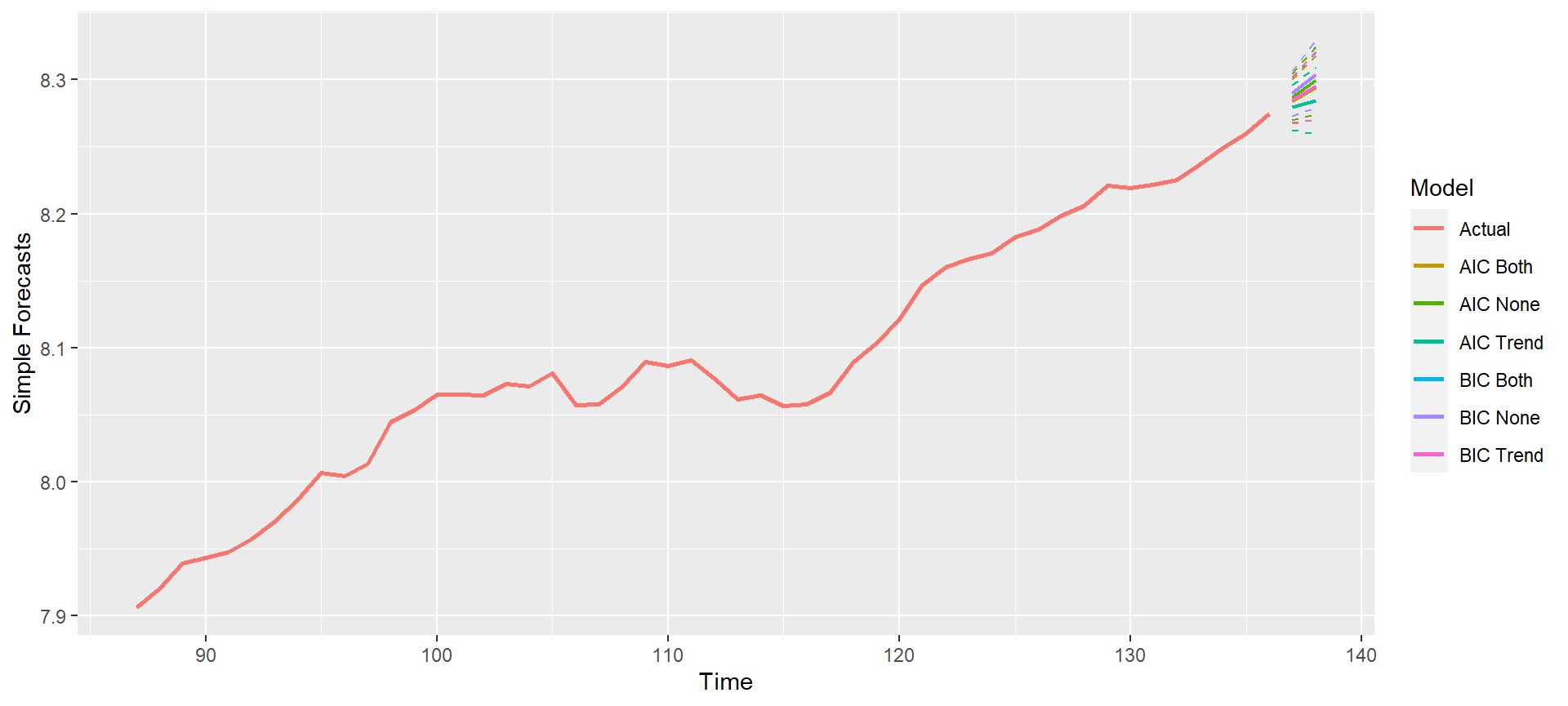
#### With n_step.ahead = TRUE (Default)              
mdl_compare = ModelCompareMultivariateVAR$new(data = data, var_interest = var_interest,
                                              mdl_list = models, n.ahead = n.ahead, batch_size = batch_size, verbose = 1)
#> Warning in private$validate_k(k, batch_size, season = mdl_list[[name]]
#> $varfit$call$season, : Although the lag value k: 10 selected by VARselect
#> will work for your full dataset, is too large for your batch size. Reducing
#> k to allow Batch ASE calculations. New k: 6 If you do not want to reduce
#> the k value, increase the batch size or make sliding_ase = FALSE for this
#> model in the model list
#> 
#> Computing metrics for:  AIC None 
#> 
#> Number of batches expected:  50
#> Computing metrics for:  AIC Trend 
#> 
#> Number of batches expected:  50
#> Computing metrics for:  AIC Both 
#> 
#> Number of batches expected:  50
#> Computing metrics for:  BIC None 
#> 
#> Number of batches expected:  50
#> Computing metrics for:  BIC Trend 
#> 
#> Number of batches expected:  50
#> Computing metrics for:  BIC Both 
#> 
#> Number of batches expected:  50# A tibble: 6 x 6
#>   Model     Trend Season SlidingASE Init_K Final_K
#>   
#> 1 AIC None  none       0 TRUE            3       3
#> 2 AIC Trend trend      0 TRUE            3       3
#> 3 AIC Both  both       0 TRUE           10       6
#> 4 BIC None  none       0 TRUE            2       2
#> 5 BIC Trend trend      0 TRUE            2       2
#> 6 BIC Both  both       0 TRUE            2       2

Compare the models

Get AIC and BIC values (trained on the complete data)

mdl_compare$get_xIC() 
#> # A tibble: 6 x 3
#>   Model        AIC    BIC
#>   
#> 1 BIC Both  -3939. -3823.
#> 2 BIC Trend -3927. -3823.
#> 3 BIC None  -3926. -3833.
#> 4 AIC Trend -3902. -3752.
#> 5 AIC None  -3901. -3763.
#> 6 AIC Both  -3701. -3224.

Compare boxplot of ASE values

p = mdl_compare$plot_boxplot_ases()

Statistically Compare the models

mdl_compare$statistical_compare()  
#>              Df    Sum Sq   Mean Sq F value  Pr(>F)    
#> Model         5 0.0000644 1.288e-05   8.523 1.5e-07 ***
#> Residuals   294 0.0004442 1.511e-06                    
#> ---
#> Signif. codes:  0 '***' 0.001 '**' 0.01 '*' 0.05 '.' 0.1 ' ' 1
#> 
#> 
#>   Tukey multiple comparisons of means
#>     95% family-wise confidence level
#> 
#> Fit: aov(formula = ASE ~ Model, data = results)
#> 
#> $Model
#>                              diff           lwr           upr     p adj
#> AIC None-AIC Both   -1.257409e-03 -0.0019626167 -0.0005522015 0.0000084
#> AIC Trend-AIC Both  -1.203493e-03 -0.0019087005 -0.0004982853 0.0000238
#> BIC Both-AIC Both   -1.209860e-03 -0.0019150679 -0.0005046527 0.0000211
#> BIC None-AIC Both   -1.292840e-03 -0.0019980477 -0.0005876326 0.0000041
#> BIC Trend-AIC Both  -1.238976e-03 -0.0019441836 -0.0005337684 0.0000120
#> AIC Trend-AIC None   5.391625e-05 -0.0006512913  0.0007591238 0.9999300
#> BIC Both-AIC None    4.754881e-05 -0.0006576588  0.0007527564 0.9999624
#> BIC None-AIC None   -3.543104e-05 -0.0007406386  0.0006697765 0.9999913
#> BIC Trend-AIC None   1.843311e-05 -0.0006867745  0.0007236407 0.9999997
#> BIC Both-AIC Trend  -6.367442e-06 -0.0007115750  0.0006988401 1.0000000
#> BIC None-AIC Trend  -8.934729e-05 -0.0007945549  0.0006158603 0.9991651
#> BIC Trend-AIC Trend -3.548314e-05 -0.0007406907  0.0006697244 0.9999912
#> BIC None-BIC Both   -8.297985e-05 -0.0007881874  0.0006222277 0.9994172
#> BIC Trend-BIC Both  -2.911570e-05 -0.0007343233  0.0006760919 0.9999967
#> BIC Trend-BIC None   5.386415e-05 -0.0006513434  0.0007590717 0.9999303
#> Call:
#>    aov(formula = ASE ~ Model, data = results)
#> 
#> Terms:
#>                        Model    Residuals
#> Sum of Squares  0.0000643868 0.0004441981
#> Deg. of Freedom            5          294
#> 
#> Residual standard error: 0.001229178
#> Estimated effects may be unbalanced

Simple Forecasts (with various options)

p = mdl_compare$plot_simple_forecasts(zoom = 50)  ## Zoom into plot

p = mdl_compare$plot_simple_forecasts(lastn = TRUE, limits = FALSE, zoom = 50)

p = mdl_compare$plot_simple_forecasts(lastn = TRUE, limits = TRUE, zoom = 50)

p = mdl_compare$plot_simple_forecasts(lastn = FALSE, limits = FALSE, zoom = 50)

p = mdl_compare$plot_simple_forecasts(lastn = FALSE, limits = TRUE, zoom = 50)

Plot and compare the forecasts per batch

p = mdl_compare$plot_batch_forecasts(only_sliding = FALSE)
#> Warning: Removed 216 row(s) containing missing values (geom_path).

#> Warning: Removed 216 row(s) containing missing values (geom_path).

#> Warning: Removed 216 row(s) containing missing values (geom_path).

Plot and compare the ASEs per batch

p = mdl_compare$plot_batch_ases() 
#> Loading required namespace: patchwork
#> Warning: Removed 216 row(s) containing missing values (geom_path).

Raw Data and Metrics

ASEs = mdl_compare$get_tabular_metrics(ases = TRUE)
print(ASEs)
#> # A tibble: 300 x 5
#>    Model          ASE Time_Test_Start Time_Test_End Batch
#>    
#>  1 AIC None 0.000685               37            38     1
#>  2 AIC None 0.000220               39            40     2
#>  3 AIC None 0.000335               41            42     3
#>  4 AIC None 0.0000418              43            44     4
#>  5 AIC None 0.000231               45            46     5
#>  6 AIC None 0.000560               47            48     6
#>  7 AIC None 0.0000166              49            50     7
#>  8 AIC None 0.0000129              51            52     8
#>  9 AIC None 0.0000701              53            54     9
#> 10 AIC None 0.000173               55            56    10
#> # ... with 290 more rows

forecasts = mdl_compare$get_tabular_metrics(ases = FALSE)
print(forecasts)
#> # A tibble: 952 x 5
#>    Model     Time     f    ll    ul
#>    
#>  1 AIC None     1    NA    NA    NA
#>  2 AIC None     2    NA    NA    NA
#>  3 AIC None     3    NA    NA    NA
#>  4 AIC None     4    NA    NA    NA
#>  5 AIC None     5    NA    NA    NA
#>  6 AIC None     6    NA    NA    NA
#>  7 AIC None     7    NA    NA    NA
#>  8 AIC None     8    NA    NA    NA
#>  9 AIC None     9    NA    NA    NA
#> 10 AIC None    10    NA    NA    NA
#> # ... with 942 more rows