1.1.2 Compare Univariate Models

Nikhil Gupta

2020-04-05

The objective of this vignette is to show how to use the ModelCompareUnivariate object to compare multiple potential models.

Setup Libraries

library(tswgewrapped)
library(tswge)
#> Warning: package 'tswge' was built under R version 3.5.3

Load Data

data("airlog")

Setup Models to be compared

# Woodward Gray Airline Model
phi_wg = c(-0.36, -0.05, -0.14, -0.11, 0.04, 0.09, -0.02, 0.02, 0.17, 0.03, -0.10, -0.38)
d_wg = 1
s_wg = 12

# Parzen Model
phi_pz = c(0.74, 0, 0, 0, 0, 0, 0, 0, 0, 0, 0, 0.38, -0.2812)
s_pz = 12

# Box Model
d_bx = 1
s_bx = 12  
theta_bx =  c(0.40, 0, 0, 0, 0, 0, 0, 0, 0, 0, 0, 0.60, -0.24)

models = list("Woodward Gray Model A" = list(phi = phi_wg, d = d_wg, s = s_wg, vara = 0.001357009, sliding_ase = FALSE),
              "Woodward Gray Model B" = list(phi = phi_wg, d = d_wg, s = s_wg, vara = 0.001357009, sliding_ase = TRUE),
              "Parzen Model A" = list(phi = phi_pz, s = s_pz, vara = 0.002933592, sliding_ase = FALSE),
              "Parzen Model B" = list(phi = phi_pz, s = s_pz, vara = 0.002933592, sliding_ase = TRUE),
              "Box Model A" = list(theta = theta_bx, d = d_bx, s = s_bx, vara = 0.001391604, sliding_ase = FALSE),
              "Box Model B" = list(theta = theta_bx, d = d_bx, s = s_bx, vara = 0.001391604, sliding_ase = TRUE)
              )

Initialize the ModelCompareUnivariate object

#### With n_step.ahead = TRUE (Default)              
mdl_compare = ModelCompareUnivariate$new(data = airlog, mdl_list = models,
                                         n.ahead = 36, batch_size = 72)
#> 
#> Batch Size has not been specified. Will assume a single batch.
#> Batch Size has not been specified. Will assume a single batch.
#> Batch Size has not been specified. Will assume a single batch.NULL

Compare the models

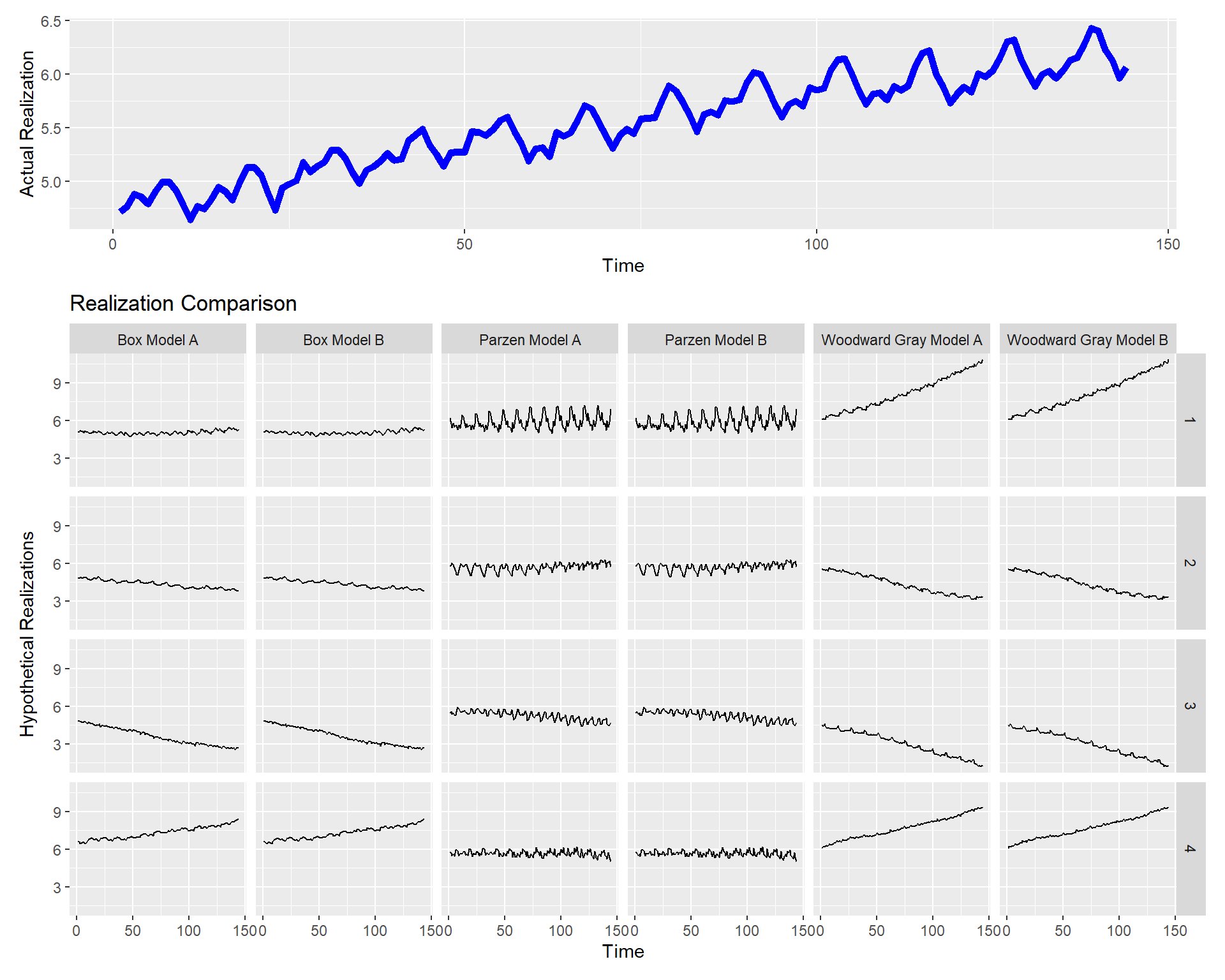
Plot Multiple realizations

p = mdl_compare$plot_multiple_realizations(n.realizations = 4, seed = 100, plot = "realization", scales = 'fixed')

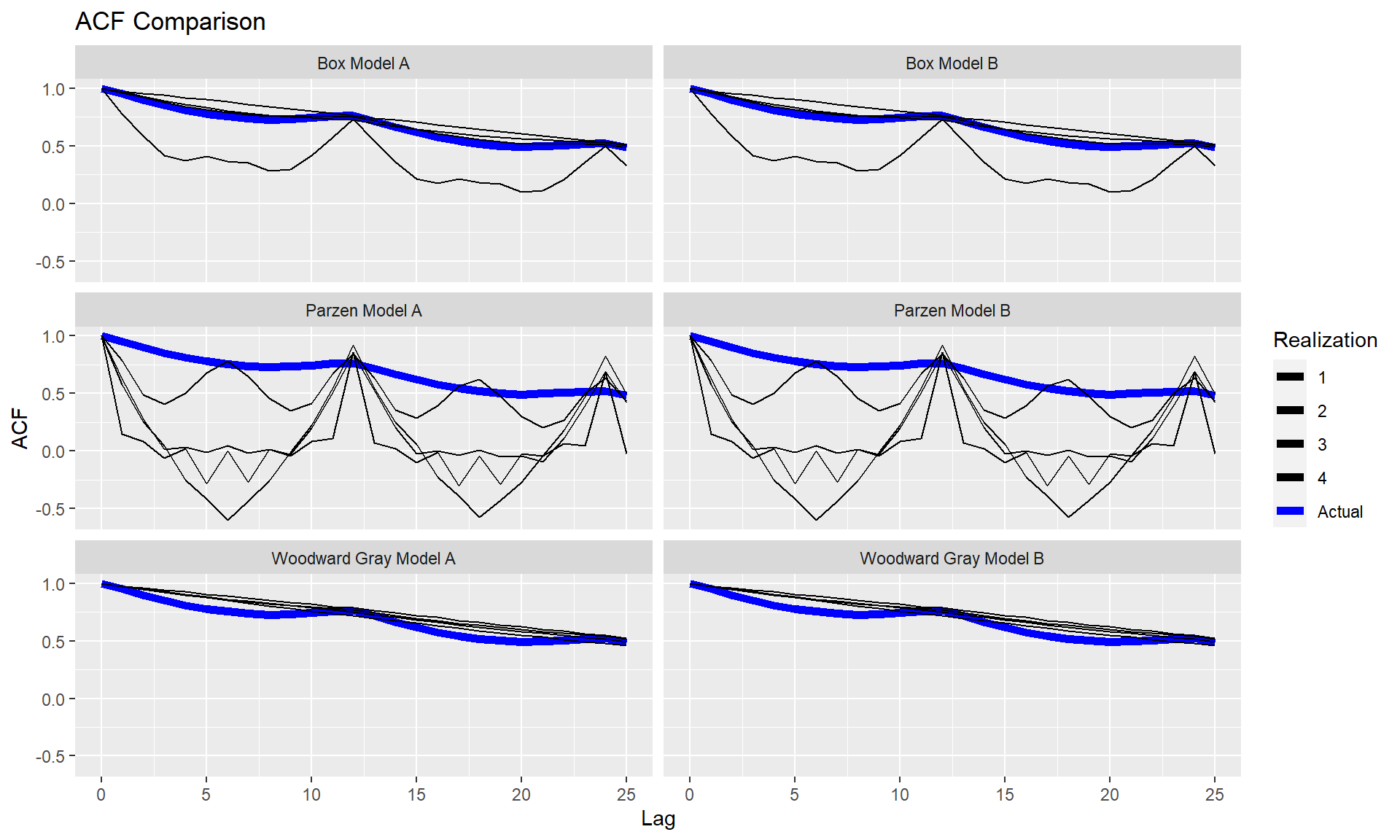
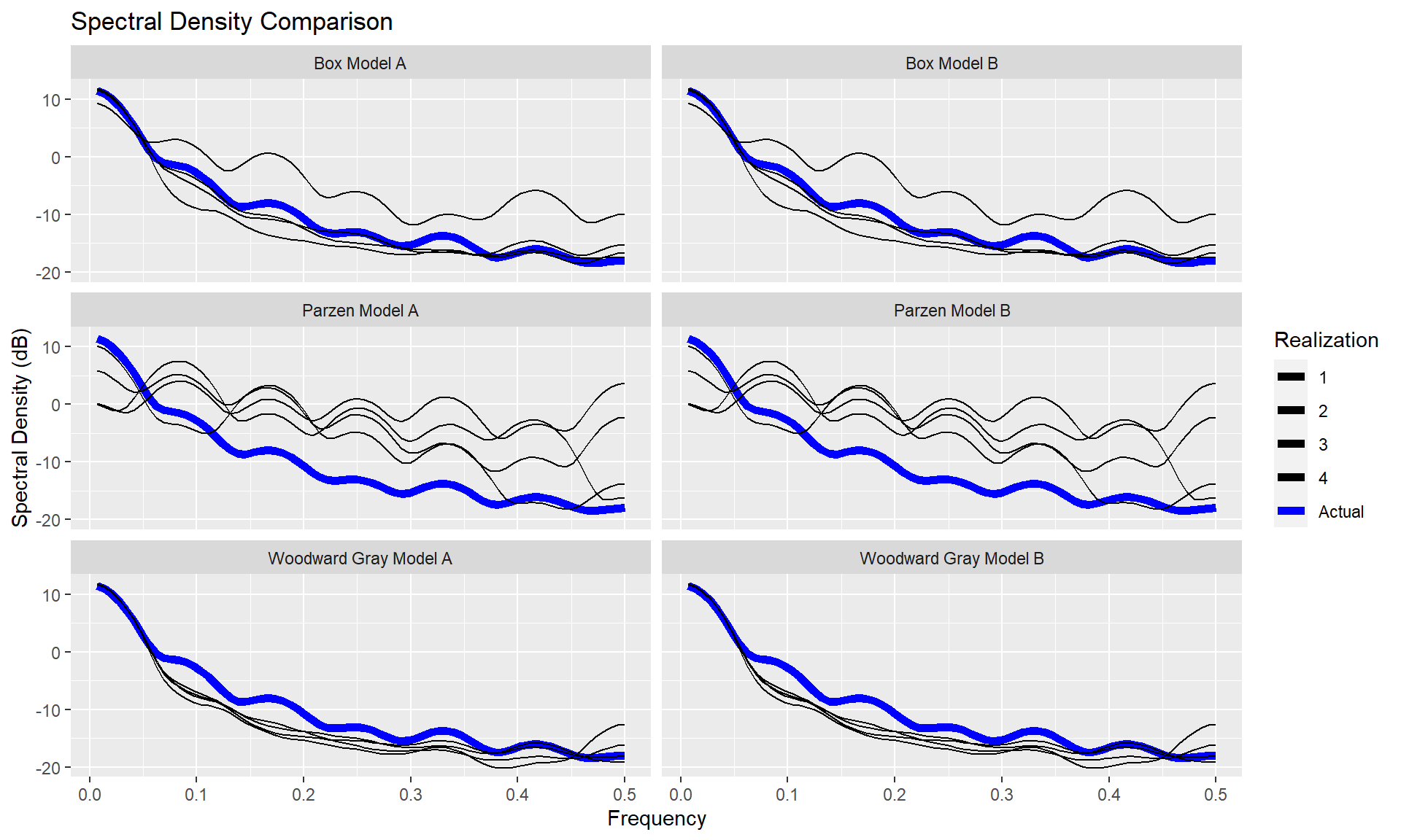
p = mdl_compare$plot_multiple_realizations(n.realizations = 4, seed = 100, plot = c("acf", "spectrum"), scales = 'fixed')

Compare boxplot of ASE values

p = mdl_compare$plot_boxplot_ases()

Statistically Compare the models

mdl_compare$statistical_compare()  
#>             Df   Sum Sq   Mean Sq F value Pr(>F)
#> Model        2 0.001460 0.0007298   2.197  0.192
#> Residuals    6 0.001993 0.0003322               
#> 
#> 
#>   Tukey multiple comparisons of means
#>     95% family-wise confidence level
#> 
#> Fit: aov(formula = ASE ~ Model, data = results)
#> 
#> $Model
#>                                              diff         lwr        upr
#> Parzen Model B-Box Model B            0.028566162 -0.01709432 0.07422664
#> Woodward Gray Model B-Box Model B     0.003429999 -0.04223048 0.04909048
#> Woodward Gray Model B-Parzen Model B -0.025136163 -0.07079665 0.02052432
#>                                          p adj
#> Parzen Model B-Box Model B           0.2134940
#> Woodward Gray Model B-Box Model B    0.9712778
#> Woodward Gray Model B-Parzen Model B 0.2838256
#> Call:
#>    aov(formula = ASE ~ Model, data = results)
#> 
#> Terms:
#>                       Model   Residuals
#> Sum of Squares  0.001459617 0.001993128
#> Deg. of Freedom           2           6
#> 
#> Residual standard error: 0.01822602
#> Estimated effects may be unbalanced

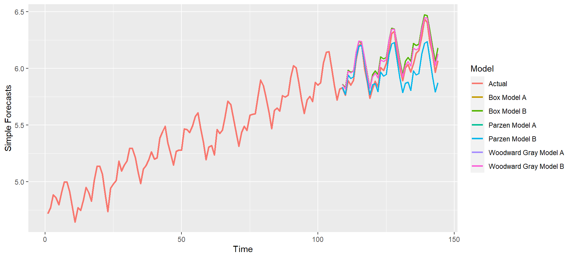
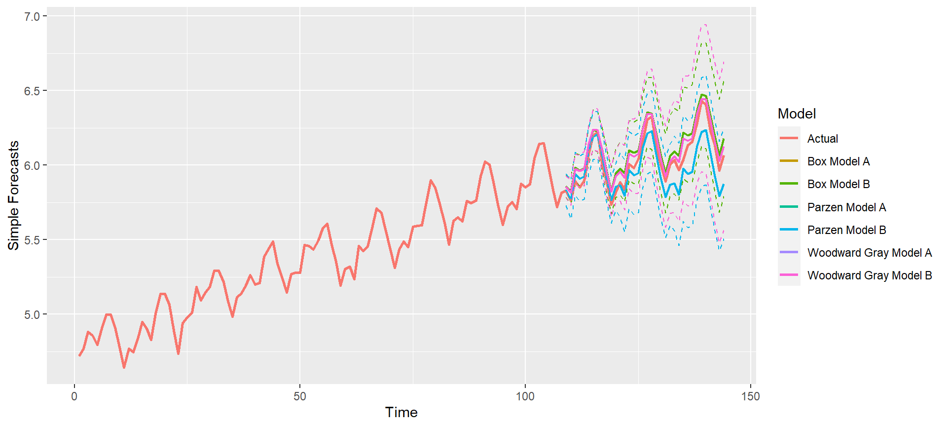
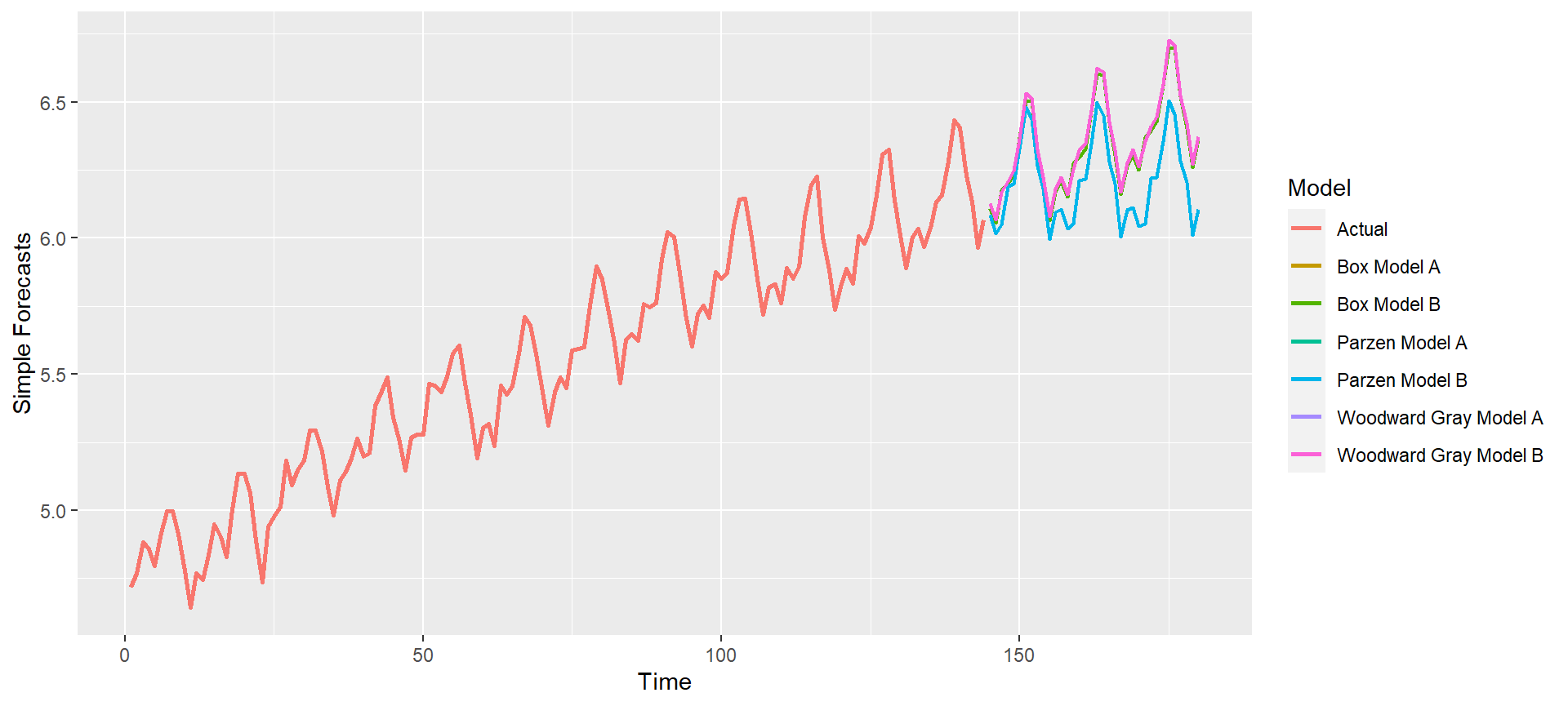
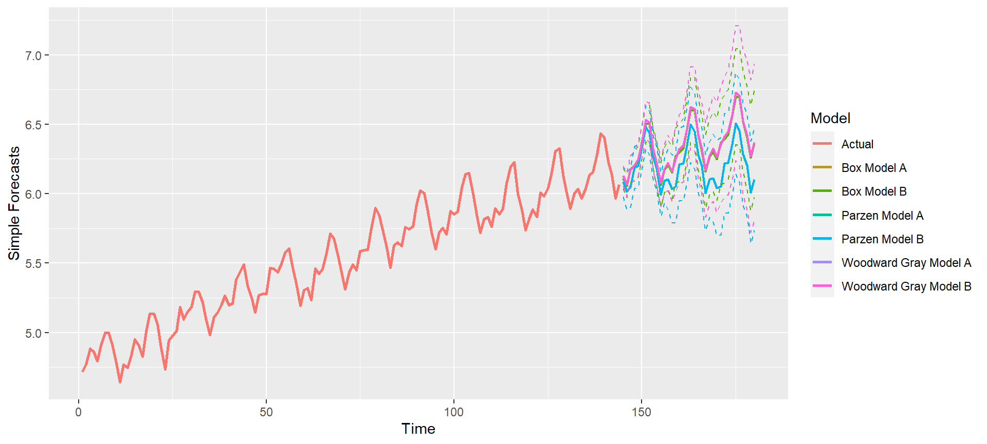
Simple Forecasts (with various options)

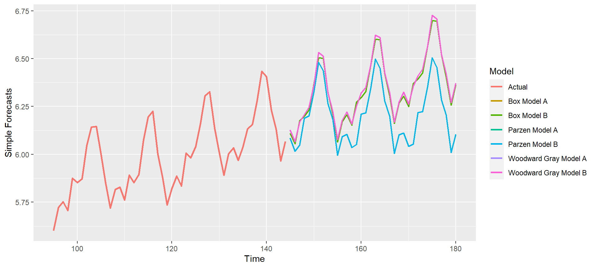
p = mdl_compare$plot_simple_forecasts(lastn = TRUE, limits = FALSE)

p = mdl_compare$plot_simple_forecasts(lastn = TRUE, limits = TRUE)

p = mdl_compare$plot_simple_forecasts(lastn = FALSE, limits = FALSE)

p = mdl_compare$plot_simple_forecasts(lastn = FALSE, limits = TRUE)

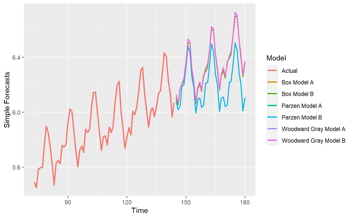
p = mdl_compare$plot_simple_forecasts(zoom = 50)  ## Zoom into plot

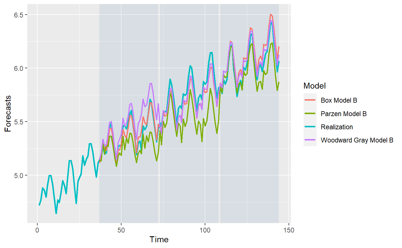
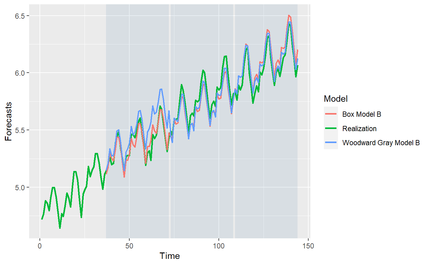
Plot and compare the forecasts per batch

p = mdl_compare$plot_batch_forecasts(only_sliding = TRUE)
#> Warning: Removed 108 row(s) containing missing values (geom_path).

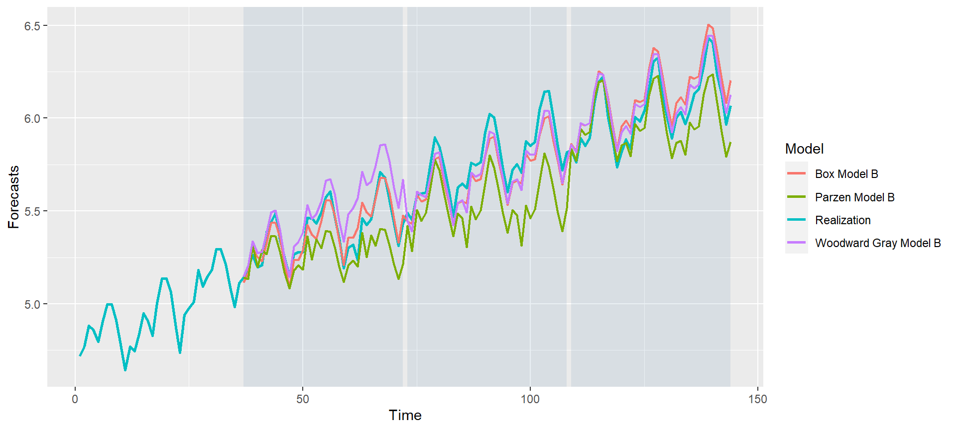
#> Warning: Removed 108 row(s) containing missing values (geom_path).

#> Warning: Removed 108 row(s) containing missing values (geom_path).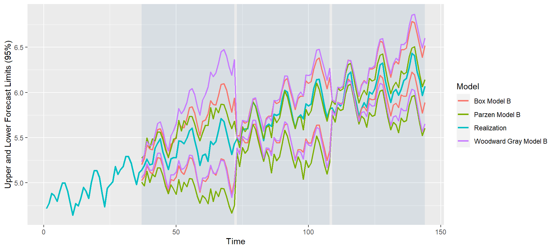

Raw Data and Metrics

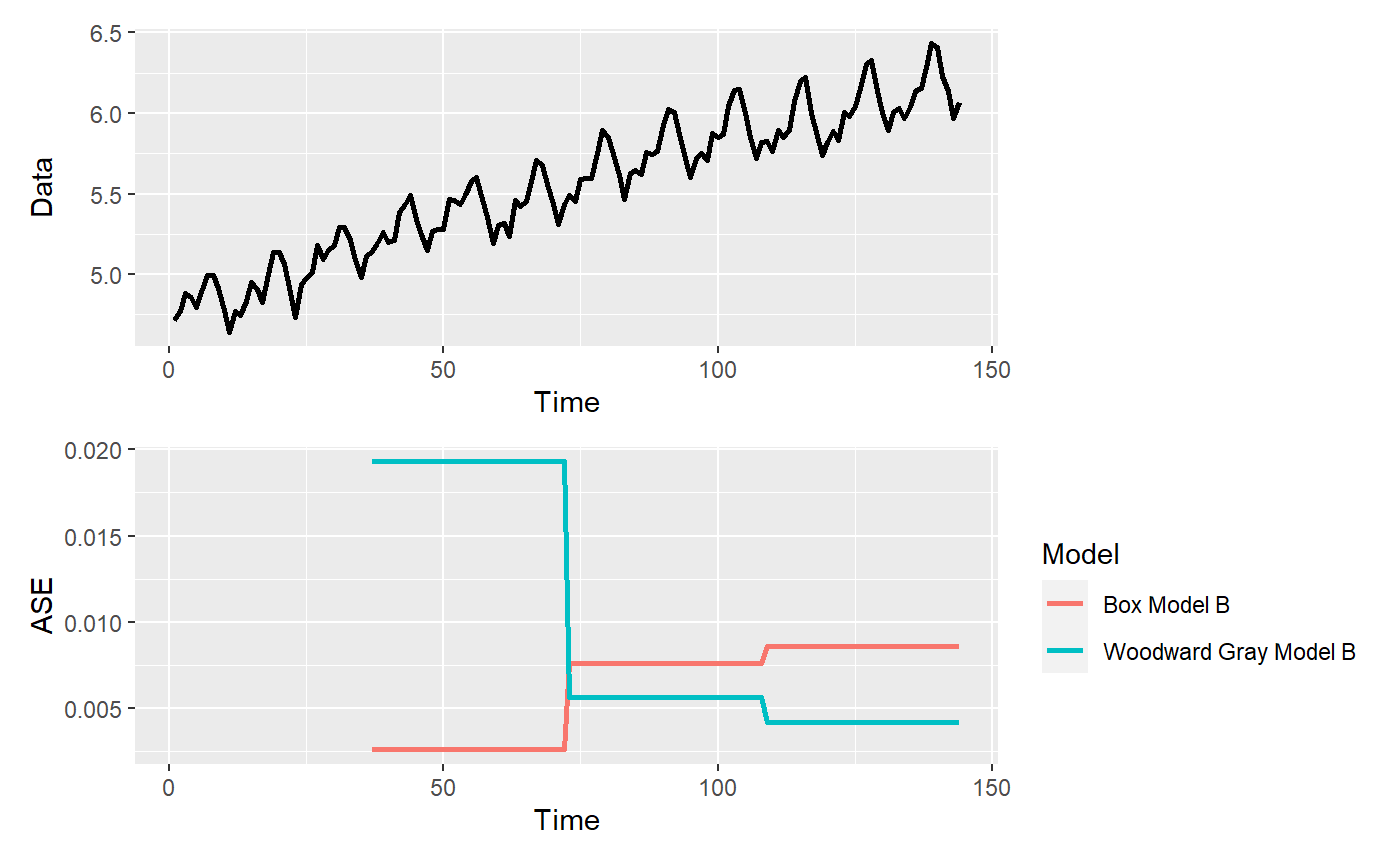
ASEs = mdl_compare$get_tabular_metrics(ases = TRUE)
print(ASEs)
#> # A tibble: 12 x 5
#>    Model                     ASE Time_Test_Start Time_Test_End Batch
#>    
#>  1 Woodward Gray Model A 0.00419             109           144     1
#>  2 Woodward Gray Model B 0.0193               37            72     1
#>  3 Woodward Gray Model B 0.00563              73           108     2
#>  4 Woodward Gray Model B 0.00419             109           144     3
#>  5 Parzen Model A        0.0125              109           144     1
#>  6 Parzen Model B        0.0227               37            72     1
#>  7 Parzen Model B        0.0693               73           108     2
#>  8 Parzen Model B        0.0125              109           144     3
#>  9 Box Model A           0.00690             109           144     1
#> 10 Box Model B           0.00261              37            72     1
#> 11 Box Model B           0.00762              73           108     2
#> 12 Box Model B           0.00862             109           144     3

forecasts = mdl_compare$get_tabular_metrics(ases = FALSE)
print(forecasts)
#> # A tibble: 1,008 x 5
#>    Model                  Time     f    ll    ul
#>    
#>  1 Woodward Gray Model A     1    NA    NA    NA
#>  2 Woodward Gray Model A     2    NA    NA    NA
#>  3 Woodward Gray Model A     3    NA    NA    NA
#>  4 Woodward Gray Model A     4    NA    NA    NA
#>  5 Woodward Gray Model A     5    NA    NA    NA
#>  6 Woodward Gray Model A     6    NA    NA    NA
#>  7 Woodward Gray Model A     7    NA    NA    NA
#>  8 Woodward Gray Model A     8    NA    NA    NA
#>  9 Woodward Gray Model A     9    NA    NA    NA
#> 10 Woodward Gray Model A    10    NA    NA    NA
#> # ... with 998 more rows

Advanced Options

Adding models after object initialization

## Add initial set of models (without sliding ASE)
models = list("Woodward Gray Model A" = list(phi = phi_wg, d = d_wg, s = s_wg, vara = 0.001357009, sliding_ase = FALSE),
              "Parzen Model A" = list(phi = phi_pz, s = s_pz, vara = 0.002933592, sliding_ase = FALSE),
              "Box Model A" = list(theta = theta_bx, d = d_bx, s = s_bx, vara = 0.001391604, sliding_ase = FALSE)
              )
  
mdl_compare = ModelCompareUnivariate$new(data = airlog, mdl_list = models,
                                         n.ahead = 36)
#> 
#> Batch Size has not been specified. Will assume a single batch.
#> Batch Size has not been specified. Will assume a single batch.
#> Batch Size has not been specified. Will assume a single batch.NULL

# Following will give an error because we are trying to add models with the same name again
# mdl_compare$add_models(mdl_list = models)

## Add models with Sliding ASE
models = list("Woodward Gray Model B" = list(phi = phi_wg, d = d_wg, s = s_wg, vara = 0.001357009, sliding_ase = TRUE),
              "Parzen Model B" = list(phi = phi_pz, s = s_pz, vara = 0.002933592, sliding_ase = TRUE),
              "Box Model B" = list(theta = theta_bx, d = d_bx, s = s_bx, vara = 0.001391604, sliding_ase = TRUE)
             )
  
# This will give warning for batch size which has not been set.
# Internally it will be set to use just 1 batch since nothing has been specified.
mdl_compare$add_models(mdl_list = models)  # This will give a warning and set only 1 batch
#> Warning in self$set_batch_size(self$get_batch_size()): You have provided
#> models that require sliding ASE calculations, but the batch size has been
#> set to NA. Setting the batch size to the length of the realization.
#> Warning in self$compute_metrics(step_n.ahead = private$get_step_n.ahead()):
#> Metrics have already been computed for Model: ' Woodward Gray Model A '.
#> These will not be computed again.
#> Warning in self$compute_metrics(step_n.ahead = private$get_step_n.ahead()):
#> Metrics have already been computed for Model: ' Parzen Model A '. These
#> will not be computed again.
#> Warning in self$compute_metrics(step_n.ahead = private$get_step_n.ahead()):
#> Metrics have already been computed for Model: ' Box Model A '. These will
#> not be computed again.
#> 
#> Batch Size has not been specified. Will assume a single batch.
#> Batch Size has not been specified. Will assume a single batch.
#> Batch Size has not been specified. Will assume a single batch.NULL
# mdl_compare$add_models(mdl_list = models, batch_size = 72)  ## This will not give a warning

Adjusting Batch Size

# If you had forgotten to set the batch size, you can do it after the fact  
mdl_compare$set_batch_size(72)
#> Warning in self$compute_metrics(step_n.ahead = private$get_step_n.ahead()):
#> Metrics have already been computed for Model: ' Woodward Gray Model A '.
#> These will not be computed again.
#> Warning in self$compute_metrics(step_n.ahead = private$get_step_n.ahead()):
#> Metrics have already been computed for Model: ' Parzen Model A '. These
#> will not be computed again.
#> Warning in self$compute_metrics(step_n.ahead = private$get_step_n.ahead()):
#> Metrics have already been computed for Model: ' Box Model A '. These will
#> not be computed again.
#> NULL


# Check all functions after data manipulation
p = mdl_compare$plot_simple_forecasts(zoom = 72)

p = mdl_compare$plot_batch_forecasts(only_sliding = TRUE)
#> Warning: Removed 108 row(s) containing missing values (geom_path).

#> Warning: Removed 108 row(s) containing missing values (geom_path).
#> Warning: Removed 108 row(s) containing missing values (geom_path).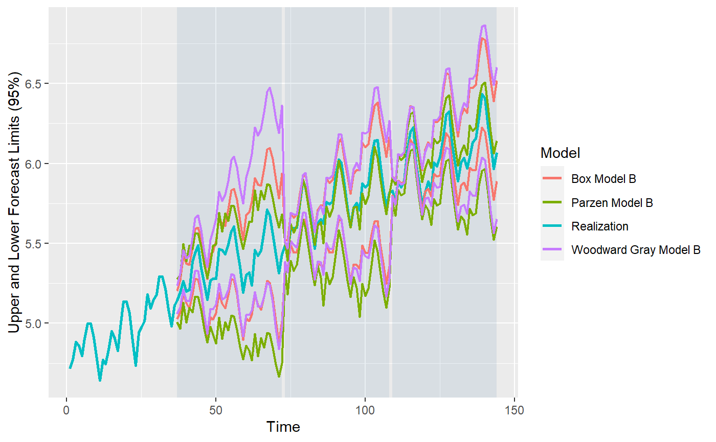

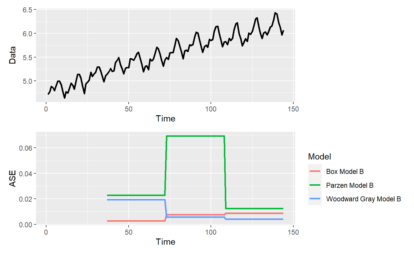
p = mdl_compare$plot_batch_ases(only_sliding = TRUE)
#> Warning: Removed 108 row(s) containing missing values (geom_path).

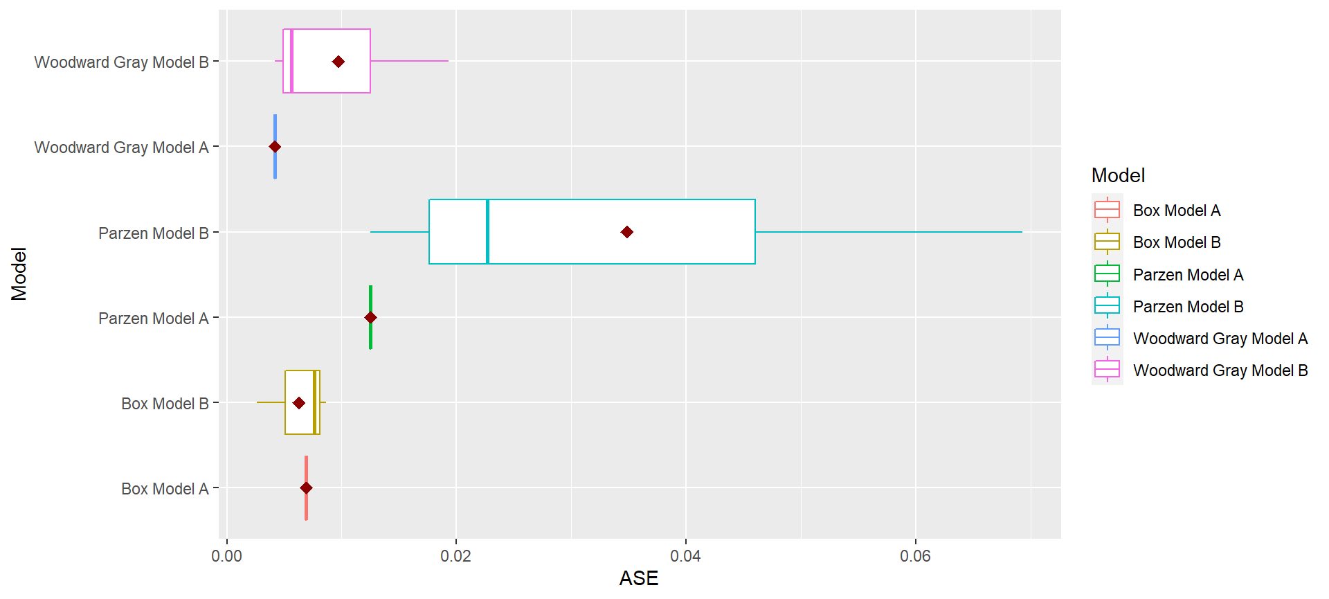
p = mdl_compare$plot_boxplot_ases()

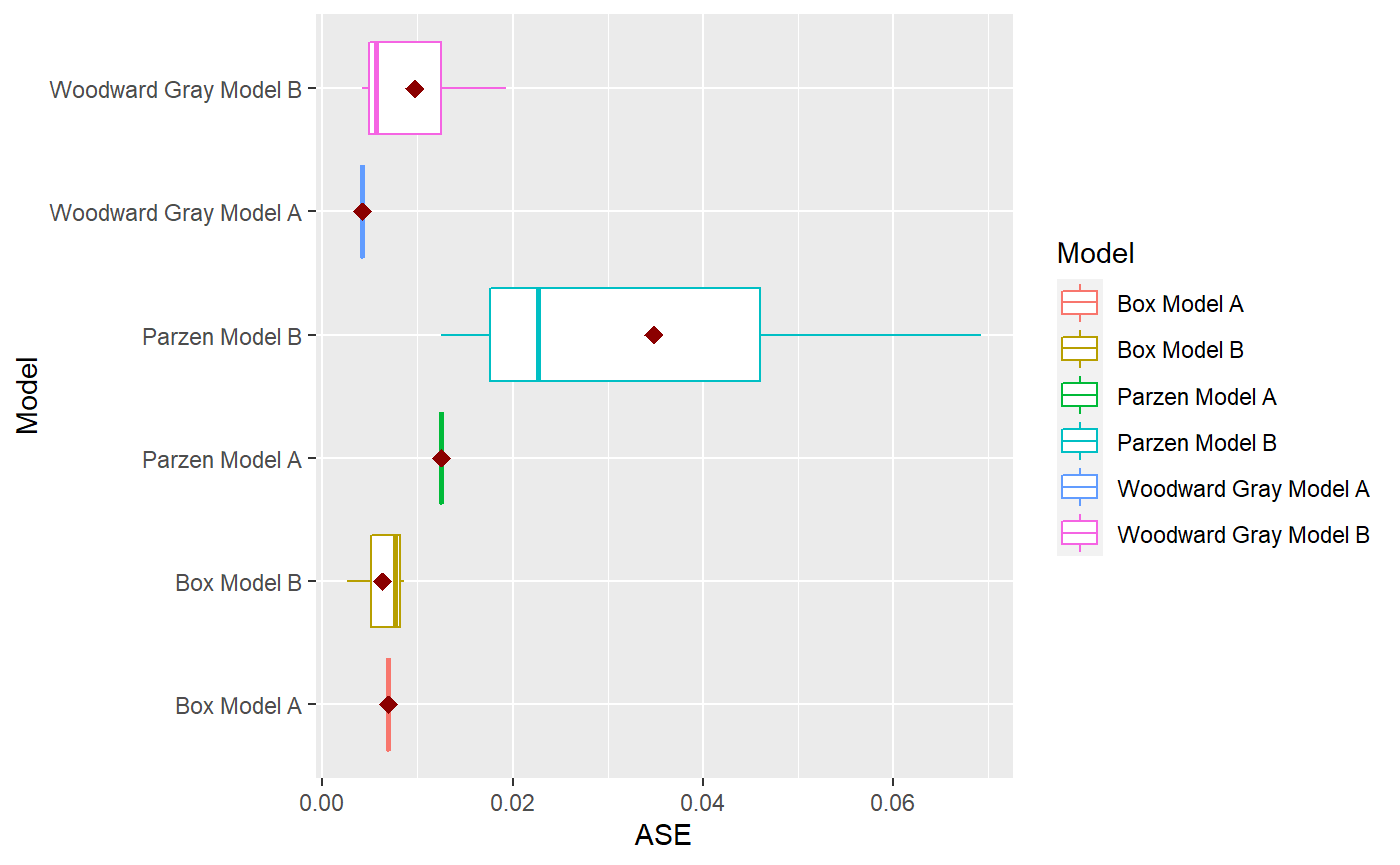
mdl_compare$statistical_compare()
#>             Df   Sum Sq   Mean Sq F value Pr(>F)
#> Model        2 0.001460 0.0007298   2.197  0.192
#> Residuals    6 0.001993 0.0003322               
#> 
#> 
#>   Tukey multiple comparisons of means
#>     95% family-wise confidence level
#> 
#> Fit: aov(formula = ASE ~ Model, data = results)
#> 
#> $Model
#>                                              diff         lwr        upr
#> Parzen Model B-Box Model B            0.028566162 -0.01709432 0.07422664
#> Woodward Gray Model B-Box Model B     0.003429999 -0.04223048 0.04909048
#> Woodward Gray Model B-Parzen Model B -0.025136163 -0.07079665 0.02052432
#>                                          p adj
#> Parzen Model B-Box Model B           0.2134940
#> Woodward Gray Model B-Box Model B    0.9712778
#> Woodward Gray Model B-Parzen Model B 0.2838256
#> Call:
#>    aov(formula = ASE ~ Model, data = results)
#> 
#> Terms:
#>                       Model   Residuals
#> Sum of Squares  0.001459617 0.001993128
#> Deg. of Freedom           2           6
#> 
#> Residual standard error: 0.01822602
#> Estimated effects may be unbalanced

Removing Unwanted Models

## After comparison, maybe you want to remove some models that are not performing well or you do not want to show in your plots
mdl_names = c("Woodward Gray Model A", "Parzen Model A", "Box Model A", "Parzen Model B")

# Remove models
mdl_compare$remove_models(mdl_names = mdl_names)
#> 
#> Model: 'Woodward Gray Model A' found in object. This will be removed.
#> Model: 'Parzen Model A' found in object. This will be removed.
#> Model: 'Box Model A' found in object. This will be removed.
#> Model: 'Parzen Model B' found in object. This will be removed.
  
# Check all functions after data manipulation
p = mdl_compare$plot_simple_forecasts()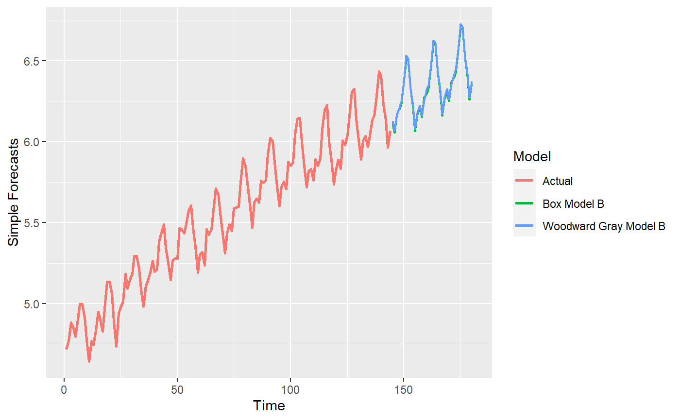

p = mdl_compare$plot_batch_forecasts()
#> Warning: Removed 72 row(s) containing missing values (geom_path).

#> Warning: Removed 72 row(s) containing missing values (geom_path).

#> Warning: Removed 72 row(s) containing missing values (geom_path).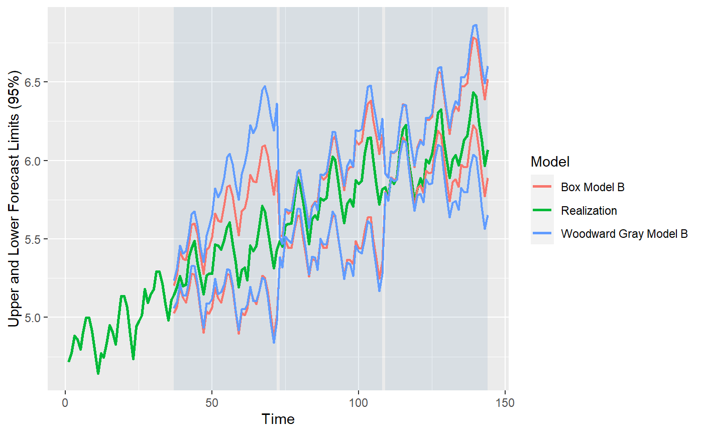

p = mdl_compare$plot_batch_ases()
#> Warning: Removed 72 row(s) containing missing values (geom_path).

p = mdl_compare$plot_boxplot_ases()

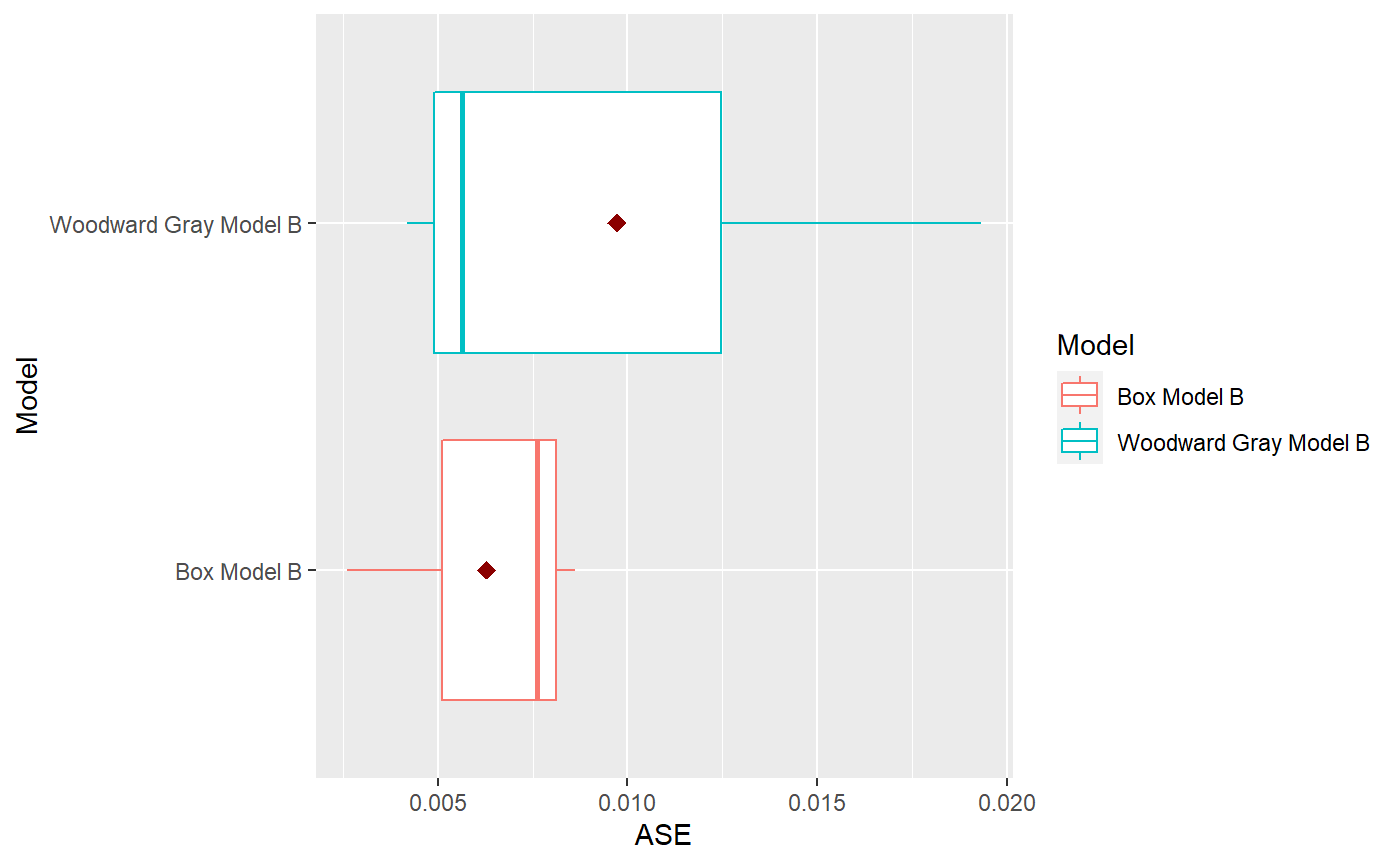
mdl_compare$statistical_compare()
#>             Df    Sum Sq   Mean Sq F value Pr(>F)
#> Model        1 1.765e-05 1.765e-05    0.44  0.543
#> Residuals    4 1.603e-04 4.008e-05               
#> 
#> 
#>   Tukey multiple comparisons of means
#>     95% family-wise confidence level
#> 
#> Fit: aov(formula = ASE ~ Model, data = results)
#> 
#> $Model
#>                                          diff         lwr        upr
#> Woodward Gray Model B-Box Model B 0.003429999 -0.01092239 0.01778238
#>                                       p adj
#> Woodward Gray Model B-Box Model B 0.5432795
#> Call:
#>    aov(formula = ASE ~ Model, data = results)
#> 
#> Terms:
#>                        Model    Residuals
#> Sum of Squares  1.764734e-05 1.603310e-04
#> Deg. of Freedom            1            4
#> 
#> Residual standard error: 0.006331094
#> Estimated effects may be unbalanced